The PostGIS development team is pleased to provide bug fix releases for PostGIS 3.0 - 3.6. These are the End-Of-Life (EOL) releases for PostGIS 3.0.12 and 3.1.13. If you haven’t already upgraded from 3.0 or 3.1 series, you should do so soon.
February 09, 2026
PostGIS Development

December 28, 2025
Boston GIS (Regina Obe, Leo Hsu)
FOSS4GNA 2025: Summary
Free and Open Source for Geospatial North America (FOSS4GNA) 2025 was running November 3-5th 2025 and I think it was one of the better FOSS4GNAs we've had. I was on the programming and workshop committees and we were worried with the government shutdown that things could go badly since we started getting people withdrawing their talks and workshops very close to curtain time. Despite our attendance being lower than prior years, it felt crowded enough and on the bright side, people weren't fighting for chairs to sit even in the most crowded talks. The FOSS4G 2025 International happened 2 weeks after, in Auckland, New Zealand, and that I heard had a fairly decent turn-out too.
Continue reading "FOSS4GNA 2025: Summary"by Regina Obe (nospam@example.com) at December 28, 2025 11:37 PM
December 09, 2025
Crunchy Data (Snowflake)

PostGIS Performance: Simplification
There’s nothing simple about simplification! It is very common to want to slim down the size of geometries, and there are lots of different approaches to the problem.
We will explore different methods starting with ST_Letters for this rendering of the letter “a”.
SELECT ST_Letters('a');
This is a good starting point, but to show the different effects of different algorithms on things like redundant linear points, we need a shape with more vertices along the straights, and fewer along the curves.
SELECT ST_RemoveRepeatedPoints(ST_Segmentize(ST_Letters('a'), 1), 1);
Here we add in vertices every one meter with ST_Segmentize and ST_RemoveRepeatedPoints to thin out the points along the curves. Already we are simplifying!
Lets apply the same “remove repeated” algorithm, with a 10 meter tolerance.
WITH a AS (
  SELECT ST_RemoveRepeatedPoints(ST_Segmentize(ST_Letters('a'), 1), 1) AS a
)
SELECT ST_RemoveRepeatedPoints(a, 10) FROM a;
We do have a lot fewer points, and the constant angle curves are well preserved, but some straight lines are no longer legible as such, and there are redundant vertices in the vertical straight lines.
The ST_Simplify function applies the Douglas-Peuker line simplification algorithm to the rings of the polygon. Because it is a line simplifier it does a cruder job preserving some aspects of the polygon area like squareness of the top ligature.
WITH a AS (
  SELECT ST_RemoveRepeatedPoints(ST_Segmentize(ST_Letters('a'), 1), 1) AS a
)
SELECT ST_Simplify(a, 1) FROM a;
The ST_SimplifyVW function applies the Visvalingam–Whyatt algorithm to the rings of the polygon. Visvalingam–Whyatt is better for preserving the shapes of polygons than Douglas-Peuker, but the differences are subtle.
WITH a AS (
  SELECT ST_RemoveRepeatedPoints(ST_Segmentize(ST_Letters('a'), 1), 1) AS a
)
SELECT ST_SimplifyVW(a, 5) FROM a;
Coercing a shape onto a fixed precision grid is another form of simplification, sometimes used to force the edges of adjacent objects to line up exactly. The original such function, ST_SnapToGrid, does exactly what it says on the name. Every vertex is rounded to a fixed grid point.
WITH a AS (
  SELECT ST_RemoveRepeatedPoints(ST_Segmentize(ST_Letters('a'), 1), 1) AS a
)
SELECT ST_SnapToGrid(a, 5) FROM a;
However, as you can see at the top left, the grid snapper frequently generates invalidity in polygons, such as the self-intersecting ring in this example.
A more modern alternative is precision reduction.
WITH a AS (
  SELECT ST_RemoveRepeatedPoints(ST_Segmentize(ST_Letters('a'), 1), 1) AS a
)
SELECT ST_ReducePrecision(a, 5) FROM a;
The ST_ReducePrecision function not only snaps geometries to a fixed precision grid, it also ensures that outputs are always valid.
Because grid snapping tends to introduce a lot of vertices along straight edges, combining it with a line simplifier makes a lot of sense.
WITH a AS (
  SELECT ST_RemoveRepeatedPoints(ST_Segmentize(ST_Letters('a'), 1), 1) AS a
)
SELECT ST_Simplify(ST_ReducePrecision(a, 5),1) FROM a;
Simplifying single geometries is all well and good, but what about simplifying groups of geometries? Specifically ones that share boundaries?
Fortunately, since PostGIS 3.6 there is now a complete set of functions for that problem.
Starting with a pair of polygons with a non-matched shared boundary.
Non-clean boundaries can be cleaned up with the ST_CoverageClean function.
SELECT ST_CoverageClean OVER() AS geom FROM polys;
And once the coverage is clean, the shapes including their shared borders can be simplified with ST_CoverageSimplify.
WITH clean AS (
  SELECT ST_CoverageClean OVER() AS geom FROM polys
)
SELECT ST_CoverageSimplify(geom, 10) OVER() FROM clean
by Paul Ramsey (Paul.Ramsey@crunchydata.com) at December 09, 2025 01:00 PM
November 21, 2025
Crunchy Data (Snowflake)
PostGIS Performance: Data Sampling
One of the temptations database users face, when presented with a huge table of interesting data, is to run queries that interrogate every record. Got a billion measurements? What’s the average of that?!
One way to find out is to just calculate the average.
SELECT avg(value) FROM mytable;
For a billion records, that could take a while!
Fortunately, the “Law of Large Numbers” is here to bail us out, stating that the average of a sample approaches the average of the population, as the sample size grows. And amazingly, the sample does not even have to be particularly large to be quite close.
Here’s a table of 10M values, randomly generated from a normal distribution. We know the average is zero. What will a sample of 10K values tell us it is?
CREATE TABLE normal AS
  SELECT random_normal(0,1) AS values
    FROM generate_series(1,10000000);
We can take a sample using a sort, or using the random() function, but both of those techniques first scan the whole table, which is exactly what we want to avoid.
Instead, we can use the PostgreSQL TABLESAMPLE feature, to get a quick sample of the pages in the table and an estimate of the average.
SELECT avg(values)
  FROM normal TABLESAMPLE SYSTEM (1);
I get an answer – 0.0031, very close to the population average – and it takes just 43 milliseconds.
Can this work with spatial? For the right data, it can. Imagine you had a table that had one point in it for every person in Canada (36 million of them) and you wanted to find out how many people lived in Toronto (or this red circle around Toronto).
SELECT count(*)
  FROM census_people
  JOIN yyz
    ON ST_Intersects(yyz.geom, census_people.geom);
The answer is 5,010,266, and it takes 7.2 seconds to return. What if we take a 10% sample?
SELECT count(*)
  FROM census_people TABLESAMPLE SYSTEM (10)
  JOIN yyz
    ON ST_Intersects(yyz.geom, census_people.geom);
The sample is 10%, and the answer comes back as 508,292 (near one tenth of our actual measurement) in 2.2 seconds. What about a 1% sample?
SELECT count(*)
  FROM census_people TABLESAMPLE SYSTEM (1)
  JOIN yyz
    ON ST_Intersects(yyz.geom, census_people.geom);
The sample is 1%, and the answer comes back as 50,379 (near one hundredth of our actual measurement) in 0.2 seconds. Still a good estimate!
Is this black magic? No, the TABLESAMPLE SYSTEM mode gets its speed by reading pages randomly. In our last example, it randomly chose 1% of the pages. Here’s what that looks like in Toronto.
See in particular how blotchy the data are in the suburban areas outside the circle. The data in the table are not randomly distributed to the pages, they came from the census data in order, and ended up loaded into the database in order. So for any given database page, the actual rows in the page will tend to be near to one another.
This works for this example because the amount of data is high, and the area we are summarizing is a large proportion of the total data – a seventh of the Canadian population lives in that circle.
If we were summarizing a smaller area, the results would not have been so good.
The TABLESAMPLE SYSTEM is a powerful tool, but you have to be sure that any given page has a random selection of the data you are sampling for. Our random normal example worked perfectly, because the data were perfectly random. A sample of time series data would not work well for sample time windows (the data were probably stored in order of arrival) but might work for sampling some other value.
by Paul Ramsey (Paul.Ramsey@crunchydata.com) at November 21, 2025 01:00 PM
November 14, 2025
Crunchy Data (Snowflake)
PostGIS Performance: Intersection Predicates and Overlays
In this series, we talk about the many different ways you can speed up PostGIS. A common geospatial operation is to clip out a collection of smaller shapes that are contained within a larger shape. Today let's review the most efficient ways to query for things inside something else.
Frequently the smaller shapes are clipped where they cross the boundary, using the ST_Intersection function.
The naive SQL is a simple spatial join on ST_Intersects.
SELECT ST_Intersection(polygon.geom, p.geom) AS geom
  FROM parcels p
  JOIN polygon
    ON ST_Intersects(polygon.geom, p.geom);
When run on the small test area shown in the pictures, the query takes about 14ms. That’s fast, but the problem is small, and larger operations will be slower.
There is a simple way to speed up the query that takes advantage of the fact that boolean spatial predicates are faster than spatial overlay operations.
What?
- “Boolean spatial predicates” are functions like ST_Intersects and ST_Contains. They take in two geometries and return “true” or “false” for whether the geometries pass the named test.
- “Spatial overlay operations” are functions like ST_Intersection or ST_Difference that take in two geometries, and generate a new geometry based on the named rule.
Predicates are faster because their tests often allow for logical short circuits (once you find any two edges that intersect, you know the geometries intersect) and because they can make use of the prepared geometry optimizations to cache and index edges between function calls.
The speed-up for spatial overlay simply observes that, for most overlays there is a large set of features that can be added to the result set unchanged – the features that are fully contained in the clipping shape. We can identify them using ST_Contains.
Similarly, there is a smaller set of features that cross the border, and thus do need to be clipped. These are features that ST_Intersects but are not ST_Contains.
The higher performance function uses the faster predicates to filter the smaller shapes into two streams, one for intersection, and one for unchanged inclusion.
SELECT
  CASE
    WHEN ST_Contains(polygon.geom, p.geom) THEN p.geom
    ELSE ST_Intersection(polygon.geom, p.geom)
    END AS geom
  FROM parcels p
  JOIN polygon
    ON ST_Intersects(polygon.geom, p.geom);
Two predicates are used here, the ST_Intersects in the join clause ensures that only parcels that might participate in the overlay are fed into the CASE statement, where the ST_Contains predicate no-ops the parcels that do not cross the boundary.
When run against our tiny example, the query executes in just 9ms. Amazing that the difference is large enough to measure on such a small example.
Using CASE statement to combine predicates and overlays
The core idea here is to recognize that boolean spatial predicates like ST_Contains and ST_Intersects are computationally much faster than spatial overlay operations like ST_Intersection. The standard, but slow, approach clips all intersecting features. The optimized method uses a CASE statement and ST_Contains check to create a shortcut: if a smaller geometry is entirely contained within the larger clipping polygon, we return the geometry unchanged (a quick no-op) and completely bypass the slower ST_Intersection calculation.
You can apply this optimization pattern to any PostGIS work involving clipping, spatial joins, or overlays where you suspect a significant number of features might be fully contained within a boundary. By filtering and partitioning your geometries into "fully contained" (fast path) and "crossing the border" (slow path) streams, you ensure the expensive overlay operations are only executed when they are strictly necessary to clip the edges.
Need more PostGIS?
Join us this year on November 20 for PostGIS Day 2025, a free, virtual, community event about open source geospatial!
by Paul Ramsey (Paul.Ramsey@crunchydata.com) at November 14, 2025 01:00 PM
November 12, 2025
PostGIS Development
PostGIS 3.6.1
The PostGIS Team is pleased to publish PostGIS 3.6.1. This is a bug fix release that includes bug fixes since PostGIS 3.6.0.
- This version requires PostgreSQL 12 - 18, Proj 6.1+, and GEOS 3.8+. To take advantage of all features, GEOS 3.12+ is needed.
- SFCGAL 1.4+ is needed to enable postgis_sfcgal support. To take advantage of all SFCGAL features, SFCGAL 2.2+ is needed.
November 06, 2025
Crunchy Data (Snowflake)
PostGIS Performance: Improve Bounding Boxes with Decompose and Subdivide
In the third installment of the PostGIS Performance series, I wanted to talk about performance around bounding boxes.
Geometry data is different from most column types you find in a relational database. The objects in a geometry column can be wildly different in the amount of the data domain they cover, and the amount of physical size they take up on disk.
The data in the “admin0” Natural Earth data range from the 1.2 hectare Vatican City, to the 1.6 billion hectare Russia, and from the 4 point polygon defining Serranilla Bank to the 68 thousand points of polygons defining Canada.
SELECT ST_NPoints(geom) AS npoints, name
FROM admin0
ORDER BY 1 DESC LIMIT 5;

SELECT ST_Area(geom::geography) AS area, name
FROM admin0
ORDER BY 1 DESC LIMIT 5;
As you can imagine, polygons this different will have different performance characteristics:
- Physically large objects will take longer to work with. To pull off the disk, to scan, to calculate with.
- Geographically large objects will cover more other objects, and reduce the effectiveness of your indexes.
Your spatial indexes are “r-tree” indexes, where each object is represented by a bounding box.
The bounding boxes can overlap, and it is possible for some boxes to cover a lot of the dataset.
For example, here is the bounding box of France.
What?! How is that France? Well, France is more than just the European parts, it also includes the island of Reunion, in the southern Indian Ocean, and the island of Guadaloupe, in the Caribbean. Taken together they result in this very large bounding box.
Such a large box makes a poor addition to the spatial index of all the objects in “admin0”. I could be searching in with a query key in the middle of the Atlantic, and the index would still be telling me “maybe it is in France?”.
For this testing, I have made a synthetic dataset of one million random points covering the whole world.
CREATE TABLE random_normal AS
  SELECT id,
    ST_Point(
      random_normal(0, 180),
      random_normal(0, 80),
      4326) AS geom
  FROM generate_series(0, 1000000) AS id;


CREATE INDEX random_normal_geom_x ON random_normal USING GIST (geom);
The un-altered bounds of “admin0”, the bounds that will be used to run the spatial join, look like this. Lots of overlap, lots of places where they bounds cover areas the polygons do not.
The baseline time to do a spatial join using the un-altered “admin0” data is 9 seconds.
SELECT Count(*), admin0.name
  FROM admin0 JOIN random_normal
    ON ST_Intersects(random_normal.geom, admin0.geom)
  GROUP BY admin0.name;
What if, instead of joining against the raw “admin0” – which includes weird cases like France and a Canada with hundreds of islands – we first decompose every object into the singular polygons that make it up, using ST_Dump.
The decomposed objects cover far less ocean, and much more accurately represent the polygons they are proxying for. And the time – including the cost of decomposing the objects – to do a full join on the 1M points falls to 3.8 seconds.
WITH polys AS  (
  SELECT (ST_Dump(geom)).geom AS geom, name
  FROM admin0
)
SELECT Count(*), polys.name
FROM polys JOIN random_normal
ON ST_Intersects(random_normal.geom, polys.geom)
GROUP BY polys.name;
There is still a lot of ocean being queried here, and also some of the polygons are not just very spatially large, but include a lot of vertices. What if we make the polygons smaller yet by chopping them up ST_Subdivide?
These bounds are almost perfect, they cover very little of the ocean, and they also have reduced the maximum memory size of any polygon to no more than 256 vertices. And the performance, even including the very expensive subdivision step, gets faster yet.
WITH polys AS (
  SELECT ST_Subdivide(geom,128) AS geom, name FROM admin0
)
SELECT Count(*), polys.name
FROM polys JOIN random_normal
ON ST_Intersects(random_normal.geom, polys.geom)
GROUP BY polys.name;
The final query takes just 1.8 seconds, twice as fast as the simple boxes, and 4 times faster than a naive spatial join. For smaller collections of points, the naive approach can work as fast as the subdivision, but for this 1M point test set the overhead of doing the subdivision is still far less than the gains from using the more effective bounds.
Investing computation into creating better, smaller, and simpler geometries pays off significantly for large datasets by making the spatial index much more effective.
Need more PostGIS?
Join us this year on November 20 for PostGIS Day 2025, a free, virtual, community event about open source geospatial!
by Paul Ramsey (Paul.Ramsey@crunchydata.com) at November 06, 2025 01:00 PM
October 27, 2025
Auchindown

Trigger Happy: Live edits in QGIS
QGIS and PostgreSQL working well together
October 20, 2025
Crunchy Data (Snowflake)
PostGIS Performance: pg_stat_statements and Postgres tuning
In this series, we talk about the many different ways you can speed up PostGIS. Today let’s talk about looking across the queries with pg_stat_statements and some basic tuning.
Showing Postgres query times with pg_stat_statements
A reasonable question to ask, if you are managing a system with variable performance is: “what queries on my system are running slowly?”
Fortunately, PostgreSQL includes an extension called “pg_stat_statements” that tracks query performance over time and maintains a list of high cost queries.
CREATE EXTENSION pg_stat_statements;
Now you will have to leave your database running for a while, so the extension can gather up data about the kind of queries that are run on your database.
Once it has been running for a while, you have a whole table – pg_stat_statements – that collects your query statistics. You can query it directly with SELECT * or you can write individual queries to find the slowest queries, the longest running ones, and so on.
Here is an example of the longest running 10 queries ranked by duration.
SELECT
  total_exec_time,
  mean_exec_time,
  calls,
  rows,
  query
FROM pg_stat_statements
WHERE calls > 0
ORDER BY mean_exec_time DESC
LIMIT 10;
While “pg_stat_statements” is good at finding individual queries to tune, and the most frequent cause of slow queries is just inefficient SQL or a need for indexing - see the first post in the series.
Occasionally performance issues do crop up at the system level. The most frequent culprit is memory pressure. PostgreSQL ships with conservative default settings for memory usage, and some workloads benefit from more memory.
Shared buffers
A database server looks like an infinite, accessible, reliable bucket of data. In fact, the server orchestrates data between the disk – which is permanent and slow – and the random access memory – which is volatile and fast – in order to provide the illusion of such a system.
When the balance between slow storage and fast memory is out of whack, system performance falls. When attempts to read data are not present in the fast memory (a “cache hit”), they continue on to the slow disk (a “cache miss”).
You can check the balance of your system by looking at the “cache hit ratio”.
SELECT
  sum(heap_blks_read) as heap_read,
  sum(heap_blks_hit)  as heap_hit,
  sum(heap_blks_hit) / (sum(heap_blks_hit) +  sum(heap_blks_read)) as ratio
FROM
  pg_statio_user_tables;
A result in the 99% is a good sign. Below 90% means that your database could be memory constrained, so increasing the “shared_buffers” parameter may help. As a general rule, “shared buffers” should be about 25% of physical RAM.
Working memory
Working memory is controlled by the “work_mem” parameter, and it controls how much memory is available for in-memory sorting, index building, and other short term processes. Unlike the “shared buffers”, which are permanent and fully allocated on startup, the “working memory” is allocated on an as-needed basis.
However, the working memory limit is applied for each database connection, so it is possible for the total working memory to radically exceed the “work_mem” value. If 1000 connections each allocate 100MB, your server will probably run out of memory.
You can speed up known memory-hungry processes, like building spatial indexes, by temporarily increasing the working memory available to your particular connection, then reduce it when the process is complete.
SET work_mem = '2GB';
CREATE INDEX roads_geom_x ON roads USING GIST (geom);
SET work_mem = '100MB';
The same principle holds for maintenance tasks, like the “VACUUM” command. You can speed up the maintenance of a large table by increasing the “maintenance_work_mem” temporarily.
SET maintenance_work_mem = '2GB';
VACUUM roads;
SET maintenance_work_mem = '128MB';
Parallelism
It is common for modern database servers to have multiple CPU cores available, but your PostgreSQL configuration may not be tuned to use them all. Postgres does have parallel query support. PostgreSQL is conservative about making use of multiple cores, because executing and coordinating multi-process queries has overheads, but in general large aggregations or scans can frequently make effective use of two to four cores at once.
Check what limits are set on your database.
SHOW max_worker_processes;

SHOW max_parallel_workers;
Setting the maximums to the number of cores on your server is good practice. In particular, don’t be afraid to reduce the number of workers if you have fewer cores – there is no benefit to be had in workers contending for cores.
Tuning Postgres basics
To wrap up:
- Check the slowest queries with pg_stat_statements.
- Use EXPLAIN and Indexing to experiment with improvements
- Check inefficient memory by looking at:
- shared buffers
- working memory (work_mem)
- parallelism
After you do some tuning, don’t forget to reset pg_stat_statements and check again to see if/how things have improved!
Need more PostGIS?
Join us this year on November 20 for PostGIS Day 2025, a free, virtual, community event about open source geospatial!
by Paul Ramsey (Paul.Ramsey@crunchydata.com) at October 20, 2025 01:00 PM
October 16, 2025
PostGIS Development
PostGIS 3.5.4
The PostGIS Team is pleased to release PostGIS 3.5.4.
This version requires PostgreSQL 12 - 18beta1, GEOS 3.8 or higher, and Proj 6.1+. To take advantage of all features, GEOS 3.12+ is needed. SFCGAL 1.4+ is needed to enable postgis_sfcgal support. To take advantage of all SFCGAL features, SFCGAL 1.5+ is needed.
- source download md5
- NEWS
- PDF docs: en
This release is a bug fix release that includes bug fixes since PostGIS 3.5.3.
October 10, 2025
Crunchy Data (Snowflake)
PostGIS Performance: Indexing and EXPLAIN
I am kicking off a short blog series on PostGIS performance fundamentals. For this first example, we will cover fundamental indexing.
We will explore performance using the Natural Earth “admin0” (countries) data (258 polygons) and their “populated places” (7342 points).
A classic spatial query is the “spatial join”, finding the relationships between objects using a spatial contain.
“How many populated places are there within each country?”
SELECT Count(*), a.name
FROM admin0 a
JOIN popplaces p
  ON ST_Intersects(a.geom, p.geom)
GROUP BY a.name ORDER BY 1 DESC;
This returns an answer, but it takes 2200 milliseconds! For two such small tables, that seems like a long time. Why?
The first stop in any performance evaluation should be the “EXPLAIN” command, which returns a detailed explanation of how the query is executed by the database.
EXPLAIN SELECT Count(*), a.name
FROM admin0 a
JOIN popplaces p
  ON ST_Intersects(a.geom, p.geom)
GROUP BY a.name;
Explain output looks complicated, but a good practice is to start from the middle (the most deeply nested) and work your way out.
                              QUERY PLAN
-------------------------------------------------------------------------
 GroupAggregate  (cost=23702129.78..23702145.38 rows=258 width=18)
   Group Key: a.name
   ->  Sort  (cost=23702129.78..23702134.12 rows=1737 width=10)
         Sort Key: a.name
         ->  Nested Loop  (cost=0.00..23702036.30 rows=1737 width=10)
               Join Filter: st_intersects(a.geom, p.geom)
               ->  Seq Scan on admin0 a  (cost=0.00..98.58 rows=258 width=34320)
               ->  Materialize  (cost=0.00..328.13 rows=7342 width=32)
                     ->  Seq Scan on popplaces p  (cost=0.00..291.42 rows=7342 width=32)
The query plan includes a minimum and maximum potential cost for each step in the plan. Steps with large differences are potential bottlenecks. Our bottleneck is in the “nested loop” join, which is performing the spatial join.
- For each geometry in the admin0 table:
- Check every geometry in the popplaces table
- If it passes the join filter, keep it in the join
- Check every geometry in the popplaces table
This pattern of checking every potential intersection is a lot of work, even for our small tables. For 258 countries and 7342 places, it runs 1.8 million intersection tests!
Just as for a non-spatial join, the key to making this query efficient is adding an index. In this case, an index on the populated places geometry.
CREATE INDEX popplaces_geom_x ON popplaces USING GIST (geom);
The PostGIS spatial index is implemented as an “r-tree” using the GIST “access method”. The “r-tree” index algorithm is auto-tuning, so you do not need to fiddle with parameters to get the best index for your data.
Important! Do not forget to specify the GIST access method with the
USING GISTkeywords in your index creation. If you leave them out, you will build a default PostgreSQL b-tree index instead, and that will provide no speed-up at all for your spatial join.
Running with the index in place, the SQL is exactly the same.
SELECT Count(*), a.name
FROM admin0 a
JOIN popplaces p
  ON ST_Intersects(a.geom, p.geom)
GROUP BY a.name;
But now it takes 200 milliseconds, 10 times faster! Why? The SQL has not changed, but thanks to the index, the query plan has changed.
                                QUERY PLAN
-----------------------------------------------------------------------------
 HashAggregate  (cost=4185.41..4187.99 rows=258 width=18)
   Group Key: a.name
   ->  Nested Loop  (cost=0.15..4176.73 rows=1737 width=10)
         ->  Seq Scan on admin0 a  (cost=0.00..98.58 rows=258 width=34320)
         ->  Index Scan using popplaces_geom_x on popplaces p  (cost=0.15..15.80 rows=1 width=32)
               Index Cond: (geom && a.geom)
               Filter: st_intersects(a.geom, geom)
The join is still a nested loop on the admin0 geometry, but instead of a sequence scan on the populated places, costing as much as 300, the inner loop is an index scan, costing only 15. As much as 20 times cheaper, resulting in our overall 10 times faster query time.
Join us this year on November 20 for PostGIS Day 2025, a free, virtual, community event about open source geospatial!
by Paul Ramsey (Paul.Ramsey@crunchydata.com) at October 10, 2025 02:00 PM
September 02, 2025
PostGIS Development
PostGIS 3.6.0
The PostGIS Team is pleased to release PostGIS 3.6.0! Best Served with PostgreSQL 18 Beta3 and recently released GEOS 3.14.0.
This version requires PostgreSQL 12 - 18beta3, GEOS 3.8 or higher, and Proj 6.1+. To take advantage of all features, GEOS 3.14+ is needed. To take advantage of all SFCGAL features, SFCGAL 2.2.0+ is needed.
-
Cheat Sheets:
This release includes bug fixes since PostGIS 3.5.3 and new features.
August 25, 2025
PostGIS Development
PostGIS 3.6.0rc2
The PostGIS Team is pleased to release PostGIS 3.6.0rc2! Best Served with PostgreSQL 18 Beta3 and recently released GEOS 3.14.0.
This version requires PostgreSQL 12 - 18beta3, GEOS 3.8 or higher, and Proj 6.1+. To take advantage of all features, GEOS 3.14+ is needed. To take advantage of all SFCGAL features, SFCGAL 2.2.0+ is needed.
-
Cheat Sheets:
This release is a beta of a major release, it includes bug fixes since PostGIS 3.5.3 and new features.
August 18, 2025
PostGIS Development
PostGIS 3.6.0rc1
The PostGIS Team is pleased to release PostGIS 3.6.0rc1! Best Served with PostgreSQL 18 Beta3 and soon to be released GEOS 3.14.
This version requires PostgreSQL 12 - 18beta3, GEOS 3.8 or higher, and Proj 6.1+. To take advantage of all features, GEOS 3.14+ is needed. To take advantage of all SFCGAL features, SFCGAL 2.2.0+ is needed.
-
Cheat Sheets:
This release is a beta of a major release, it includes bug fixes since PostGIS 3.5.3 and new features.
August 01, 2025
Auchindown
The Beauty of Extensibility
You don't always have to wait for new functionality, you can sometimes do it yourself
July 20, 2025
PostGIS Development
PostGIS 3.6.0rc1
The PostGIS Team is pleased to release PostGIS 3.6.0rc1! Best Served with PostgreSQL 18 Beta3 and soon to be released GEOS 3.14.
This version requires PostgreSQL 12 - 18beta3, GEOS 3.8 or higher, and Proj 6.1+. To take advantage of all features, GEOS 3.14+ is needed. To take advantage of all SFCGAL features, SFCGAL 2.2.0+ is needed.
-
Cheat Sheets:
This release is a beta of a major release, it includes bug fixes since PostGIS 3.5.3 and new features.
PostGIS Development
PostGIS 3.6.0beta1
The PostGIS Team is pleased to release PostGIS 3.6.0beta1! Best Served with PostgreSQL 18 Beta2 and soon to be released GEOS 3.14.
This version requires PostgreSQL 12 - 18beta2, GEOS 3.8 or higher, and Proj 6.1+. To take advantage of all features, GEOS 3.14+ is needed. To take advantage of all SFCGAL features, SFCGAL 2.2.0+ is needed.
-
Cheat Sheets:
This release is a beta of a major release, it includes bug fixes since PostGIS 3.5.3 and new features.
May 18, 2025
PostGIS Development
PostGIS 3.6.0alpha1
The PostGIS Team is pleased to release PostGIS 3.6.0alpha1! Best Served with PostgreSQL 18 Beta1 and GEOS 3.13.1.
This version requires PostgreSQL 12 - 18beta1, GEOS 3.8 or higher, and Proj 6.1+. To take advantage of all features, GEOS 3.12+ is needed. To take advantage of all SFCGAL features, SFCGAL 2.1.0+ is needed.
-
Cheat Sheets:
This release is an alpha of a major release, it includes bug fixes since PostGIS 3.5.3 and new features.
May 17, 2025
PostGIS Development
PostGIS 3.5.3
The PostGIS Team is pleased to release PostGIS 3.5.3.
This version requires PostgreSQL 12 - 18beta1, GEOS 3.8 or higher, and Proj 6.1+. To take advantage of all features, GEOS 3.12+ is needed. SFCGAL 1.4+ is needed to enable postgis_sfcgal support. To take advantage of all SFCGAL features, SFCGAL 1.5+ is needed.
-
PDF docs: en
-
Cheat Sheets:
This release is a bug fix release that includes bug fixes since PostGIS 3.5.1.
March 14, 2025
Crunchy Data (Snowflake)
Pi Day PostGIS Circles
What's your favourite infinite sequence of non-repeating digits? There are some people who make a case for e, but to my mind nothing beats the transcendental and curvy utility of π, the ratio of a circle's circumference to its diameter.
Drawing circles is a simple thing to do in PostGIS -- take a point, and buffer it. The result is circular, and we can calculate an estimate of pi just by measuring the perimeter of the unit circle.
SELECT ST_Buffer('POINT(0 0)', 1.0);
Except, look a little more closely -- this "circle" seems to be made up of short straight lines. What is the ratio of its circumference to its diameter?
SELECT ST_Perimeter(ST_Buffer('POINT(0 0)', 1.0)) / 2;
3.1365484905459406
That's close to pi, but it's not pi. Can we generate a better approximation? What if we make the edges even shorter? The third parameter to ST_Buffer() is the "quadsegs", the number of segments to build each quadrant of the circle.
SELECT ST_Perimeter(ST_Buffer('POINT(0 0)', 1.0, quadsegs => 128)) / 2;
3.1415729403671087
Much closer!
We can crank this process up a lot more, keep adding edges, but at some point the process becomes silly. We should just be able to say "this edge is a portion of a circle, not a straight line", and get an actual circular arc.
Good news, we can do exactly that! The CIRCULARSTRING is the curvy analogue to a LINESTRING wherein every connection is between three points that define a portion of a circle.
The circular arc above is the arc that starts at A and ends at C, passing through B. Any three points define a unique circular arc. A CIRCULARSTRING is a connected sequence of these arcs, just as a LINESTRING is a connected sequence of linear edges.
How does this help us get to pi though? Well, PostGIS has a moderate amount of support for circular arc geometry, so if we construct a circle using "natively curved" objects, we should get an exact representation of a circle rather than an approximation.
So, what is an arc that starts and ends at the same point? A circle! This is the unit circle -- a circle of radius one centered on the origin -- expressed as a CIRCULARSTRING.
SELECT ST_Length('CIRCULARSTRING(1 0, -1 0, 1 0)') / 2;
3.141592653589793
That looks a lot like pi!
Let's bust out the built-in pi() function from PostgreSQL and check to be sure.
SELECT pi() - ST_Length('CIRCULARSTRING(1 0, -1 0, 1 0)') / 2;
0
Yep, a perfect π to celebrate "Pi Day" with!
by Paul Ramsey (Paul.Ramsey@crunchydata.com) at March 14, 2025 02:00 PM
February 10, 2025
Paul Ramsey

The Early History of Spatial Databases and PostGIS
For PostGIS Day this year I researched a little into one of my favourite topics, the history of relational databases. I feel like in general we do not pay a lot of attention to history in software development. To quote Yoda, “All his life has he looked away… to the future, to the horizon. Never his mind on where he was. Hmm? What he was doing.”
Anyways, this year I took on the topic of the early history of spatial databases in particular. There was a lot going on in the ’90s in the field, and in many ways PostGIS was a late entrant, even though it gobbled up a lot of the user base eventually.
February 07, 2025
Crunchy Data (Snowflake)
Using Cloud Rasters with PostGIS
With the postgis_raster extension, it is possible to access gigabytes of raster data from the cloud, without ever downloading the data.
How? The venerable postgis_raster extension (released 13 years ago) already has the critical core support built-in!
Rasters can be stored inside the database, or outside the database, on a local file system or anywhere it can be accessed by the underlying GDAL raster support library. The storage options include S3, Azure, Google, Alibaba, and any HTTP server that supports RANGE requests.
As long as the rasters are in the cloud optimized GeoTIFF (aka "COG") format, the network access to the data will be optimized and provide access performance limited mostly by the speed of connection between your database server and the cloud storage.
TL;DR It Works
Prepare the Database
Set up a database named raster with the postgis and postgis_raster extensions.
CREATE EXTENSION postgis;
CREATE EXTENSION postgis_raster;

ALTER DATABASE raster
  SET postgis.gdal_enabled_drivers TO 'GTiff';

ALTER DATABASE raster
  SET postgis.enable_outdb_rasters TO true;
Investigate The Data
COG is still a new format for public agencies, so finding a large public example can be tricky. Here is a 56GB COG of medium resolution (30m) elevation data for Canada. Don't try and download it, it's 56GB!
You can see some metadata about the file using the gdalinfo utility to read the headers.
gdalinfo /vsicurl/https://datacube-prod-data-public.s3.amazonaws.com/store/elevation/mrdem/mrdem-30/mrdem-30-dsm.tif
Note that we prefix the URL to the image with /viscurl/ to tell GDAL to use virtual file system access rather than direct download.
There is a lot of metadata!
Metadata from gdalinfo
Driver: GTiff/GeoTIFF
Files: /vsicurl/https://datacube-prod-data-public.s3.amazonaws.com/store/elevation/mrdem/mrdem-30/mrdem-30-dsm.tif
Size is 183687, 159655
Coordinate System is:
PROJCRS["NAD83(CSRS) / Canada Atlas Lambert",
    BASEGEOGCRS["NAD83(CSRS)",
        DATUM["NAD83 Canadian Spatial Reference System",
            ELLIPSOID["GRS 1980",6378137,298.257222101,
                LENGTHUNIT["metre",1]]],
        PRIMEM["Greenwich",0,
            ANGLEUNIT["degree",0.0174532925199433]],
        ID["EPSG",4617]],
    CONVERSION["Canada Atlas Lambert",
        METHOD["Lambert Conic Conformal (2SP)",
            ID["EPSG",9802]],
        PARAMETER["Latitude of false origin",49,
            ANGLEUNIT["degree",0.0174532925199433],
            ID["EPSG",8821]],
        PARAMETER["Longitude of false origin",-95,
            ANGLEUNIT["degree",0.0174532925199433],
            ID["EPSG",8822]],
        PARAMETER["Latitude of 1st standard parallel",49,
            ANGLEUNIT["degree",0.0174532925199433],
            ID["EPSG",8823]],
        PARAMETER["Latitude of 2nd standard parallel",77,
            ANGLEUNIT["degree",0.0174532925199433],
            ID["EPSG",8824]],
        PARAMETER["Easting at false origin",0,
            LENGTHUNIT["metre",1],
            ID["EPSG",8826]],
        PARAMETER["Northing at false origin",0,
            LENGTHUNIT["metre",1],
            ID["EPSG",8827]]],
    CS[Cartesian,2],
        AXIS["(E)",east,
            ORDER[1],
            LENGTHUNIT["metre",1]],
        AXIS["(N)",north,
            ORDER[2],
            LENGTHUNIT["metre",1]],
    USAGE[
        SCOPE["Transformation of coordinates at 5m level of accuracy."],
        AREA["Canada - onshore and offshore - Alberta; British Columbia; Manitoba; New Brunswick; Newfoundland and Labrador; Northwest Territories; Nova Scotia; Nunavut; Ontario; Prince Edward Island; Quebec; Saskatchewan; Yukon."],
        BBOX[38.21,-141.01,86.46,-40.73]],
    ID["EPSG",3979]]
Data axis to CRS axis mapping: 1,2
Origin = (-2454000.000000000000000,3887400.000000000000000)
Pixel Size = (30.000000000000000,-30.000000000000000)
Metadata:
  TIFFTAG_DATETIME=2024:05:08 12:00:00
  AREA_OR_POINT=Area
Image Structure Metadata:
  LAYOUT=COG
  COMPRESSION=LZW
  INTERLEAVE=BAND
Corner Coordinates:
Upper Left  (-2454000.000, 3887400.000) (175d38'57.51"W, 68d 7'32.00"N)
Lower Left  (-2454000.000, -902250.000) (121d27'11.17"W, 36d35'36.71"N)
Upper Right ( 3056610.000, 3887400.000) ( 10d43'16.37"W, 62d45'36.29"N)
Lower Right ( 3056610.000, -902250.000) ( 63d 0'39.68"W, 34d21' 6.31"N)
Center      (  301305.000, 1492575.000) ( 88d57'23.39"W, 62d31'56.78"N)
Band 1 Block=512x512 Type=Float32, ColorInterp=Gray
  NoData Value=-32767
  Overviews: 91843x79827, 45921x39913, 22960x19956, 11480x9978, 5740x4989, 2870x2494, 1435x1247, 717x623, 358x311
The key things we need to take from the metadata are that:
- the spatial reference system is "NAD83(CSRS) / Canada Atlas Lambert", "EPSG:3979"; and,
- the blocking (tiling) is 512x512 pixels.
Load The Database Table
With this metadata in hand, we are ready to load a reference to the remote data into our database, using the raster2pgsql utility that comes with PostGIS.
./raster2pgsql \
  -R \
  -k \
  -s 3979 \
  -t 512x512 \
  -Y 1000 \
  /vsicurl/https://datacube-prod-data-public.s3.amazonaws.com/store/elevation/mrdem/mrdem-30/mrdem-30-dsm.tif \
  mrdem30 \
  | psql raster
That is a lot of flags! What do they mean?
- -R means store references, so the pixel data is not copied into the database.
- -k means do not skip tiles that are all NODATA values. While it would be nice to skip NODATA tiles, doing so involves reading all the pixel data, which is exactly what we are trying to avoid.
- -s 3979 means that the projection of our data is EPSG:3979, the value we got from the metadata.
- -t 512x512 means to create tiles with 512x512 pixels, so that the blocking of the tiles in our database matches the blocking of the remote file. This should help lower the number of network reads any given data request requires.
- -Y 1000 means to use
COPYmode when writing out the tile definitions, and to write out batches of 1000 rows in eachCOPYblock. - Then the URL to the cloud GeoTIFF we are referencing, with
/vsicurl/at the front to indicate using the "curl virtual file system". - Then the table name (
mrdem30) we want to use in the database. - Finally we pipe the result of the command (which is just SQL text) to
psqlto load it into therasterdatabase.
When we are done, we have a table of raster tiles that looks like this in the database.
                     Table "public.mrdem30"
 Column |  Type   | Nullable |               Default
--------+---------+-----------+----------+--------------------------------------
 rid    | integer | not null | nextval('mrdem30_rid_seq'::regclass)
 rast   | raster  |          |
Indexes:
    "mrdem30_pkey" PRIMARY KEY, btree (rid)
We should add a geometry index on the raster column, specifically on the bounds of each tile.
CREATE INDEX mrdem30_st_convexhull_idx
  ON mrdem30 USING GIST (ST_ConvexHull(rast));
This index will speed up the raster tile lookup needed when we are spatially querying.
Query The Data
The single MrDEM GeoTIFF data set is now represented in the database as a table of raster tiles.
SELECT count(*) FROM mrdem30;
There are 112008 tiles in the collection.
Each tile is pretty big, spatially (512 pixels on a side, 30 meters per pixel, means a 15km tile).
Each tile knows what file it references, where it is on the globe and what projection it is in.
SELECT (ST_BandMetadata(rast)).*
  FROM mrdem30 OFFSET 50000 LIMIT 1;
pixeltype     | 32BF
nodatavalue   | -32767
isoutdb       | t
path          | /vsicurl/https://datacube-prod-data-public.s3.amazonaws.com/store/elevation/mrdem/mrdem-30/mrdem-30-dsm.tif
outdbbandnum  | 1
filesize      | 59659542216
filetimestamp | 1718629812
The ST_ConvexHull() function can be used to get a polygon geometry of the raster bounds.
SELECT ST_AsText(ST_ConvexHull(rast))
  FROM mrdem30 OFFSET 50000 LIMIT 1;
POLYGON((-2054640 -367320,-2039280 -367320,-2039280 -382680,-2054640 -382680,-2054640 -367320))
Just like geometries, raster tiles have a spatial reference id associated with them, in this case a projection that makes sense for a Canada-wide raster.
SELECT ST_SRID(rast)
  FROM mrdem30 OFFSET 50000 LIMIT 1;
3979
Query Elevation
So how do we get an elevation value from this collection of reference tiles? Easy! For any given point, we pull the tile that point falls inside, and then read off the elevation at that point.
-- Make point for Toronto
-- Transform to raster coordinate system
WITH pt AS (
  SELECT ST_Transform(
    ST_Point(-79.3832, 43.6532, 4326),
    3979) AS toronto
)
-- Find the raster tile of interest,
-- and read the value of band one (there is only one band)
-- at that point.
SELECT
  ST_Value(rast, 1, toronto, resample => 'bilinear') AS elevation,
  toronto AS geom
FROM
  mrdem30, pt
WHERE ST_Intersects(ST_ConvexHull(rast), toronto);
Note that we are using "bilinear interpolation" in ST_Value(), so if our point falls between pixel values, the value we get is interpolated in between the pixel values.
Query a Larger Geometry
What about something bigger? How about the flight line of a plane going from Victoria (YYJ) to Calgary (YYC) over the Rocky Mountains?
- Generate the points
- Make a flight route to join them
- Transform that route into the coordinate system of the raster
- Pull all the rasters that touch the line and merge them into one giant raster in memory
- Copy the values off the raster into the Z coordinate of the line
- Dump the line into points to make a pretty picture
-- Create start and end points of route
-- YYJ = Victoria, YYC = Calgary
CREATE TABLE flight AS
WITH
end_pts AS (
    SELECT ST_Point(-123.3656, 48.4284, 4326) AS yyj,
           ST_Point(-114.0719, 51.0447, 4326) AS yyc
),
-- Construct line and add vertex every 10KM along great circle
-- Reproject to coordinate system of rasters
ln AS (
    SELECT ST_Transform(ST_Segmentize(
        ST_MakeLine(end_pts.yyj, end_pts.yyc)::geography,
        10000)::geometry, 3979) AS geom
    FROM end_pts
),
rast AS (
    SELECT ST_Union(rast) AS r
    FROM mrdem30, ln
    WHERE ST_Intersects(ST_ConvexHull(rast), ln.geom)
),
-- Add Z values to that line
zln AS (
    SELECT ST_SetZ(rast.r, ln.geom) AS geom
    FROM rast, ln
),
-- Dump the points of the line for the graph
zpts AS (
    SELECT (ST_DumpPoints(geom)).*
    FROM zln
)
SELECT geom, ST_Z(geom) AS elevation
FROM zpts;
From the elevated points, we can make a map showing the flight line, and the elevations along the way.
Why does it work?
How is it possible to read the values off of a 56GB GeoTIFF file without ever downloading the file?
Cloud Optimized GeoTIFF
The difference between a "cloud GeoTIFF" and a "local GeoTIFF" is mostly a difference in how software accesses the data.
A local GeoTIFF probably resides on an SSD or some other storage that has fast random access. Small random reads will be fast, and so will large sequential reads. Local access is fast!
A cloud GeoTIFF resides on an "object store", a remote API that allows clients to real all of a file (with an HTTP "GET") or part of a file (with an HTTP "RANGE"). Each random read is quite slow, because the read involves setting up an HTTP connection (slow) and then transmitting the data over an internetwork (slow). The more reads you do, the worse performance get. So the core goal of a "cloud format" is to reduce the number of reads required to access a subset of the data.
Reading multi-gigabyte raster files from object storage is a relatively new idea, formalized only a couple years ago in the cloud optimized GeoTIFF (aka COG) specification.
The "cloud optimization" takes the form of just a few restrictions on the ordinary GeoTIFF:
- Pixel data are tiled
- Overviews are also tiled
Forcing tiling means that pixels that are near each other in space are also near each other in the file. Pixels that are near each other in the file can be read in a single read, which is great when you are reading from cloud object storage.
(Another "cloud format" shaking up the industry is Parquet, and Crunchy Data Warehouse can do direct access and query on Parquet for precisely the same reasons that postgis_raster can query COG files -- the format is structured to reduce the number of reads needed to carry out common queries.)
GDAL Virtual File Systems
While a "cloud optimized" format like COG or GeoParquet is cool, it is not going to be a useful cloud format without a client library that knows how to efficiently read the file. The client needs to be native to the application, and it needs to be parsimonious in the number of file accesses it makes.
For a web application, that means that COG access requires a JavaScript library that understands the GeoTIFF format.
For a database written in C, like PostgreSQL/PostGIS, that means that access requires a C/C++ library that understands GeoTIFF and abstracts file system operations, so that the GeoTIFF reader can support both local file system access and remote cloud access.
For PostGIS raster, that library is GDAL. Every build of postgis_raster is linked to GDAL and allows us to take advantage of the library capabilities.
GDAL allows direct access to COG files on remote cloud storage services.
- Any HTTP server that supports Range requests
- AWS S3
- Google Cloud Storage
- Azure Blob Storage
- and others!
The specific cloud service support allows things like access keys to be used for reading private objects. There is more information about accessing secure buckets with PostGIS raster in this blog post.
Under the covers GDAL not only reads COG format files, it also maintains a modest in-memory data cache. This means there's a performance premium to making sure your raster queries are spatially coherent (each query point is near the previous one) because this maximizes the use of cached data.
by Paul Ramsey (Paul.Ramsey@crunchydata.com) at February 07, 2025 03:30 PM
February 03, 2025
Paul Ramsey
WKB EMPTY
I have been watching the codification of spatial data types into GeoParquet and now GeoIceberg with some interest, since the work is near and dear to my heart.
Writing a disk serialization for PostGIS is basically an act of format standardization – albeit a standard with only one consumer – and many of the same issues that the Parquet and Iceberg implementations are thinking about are ones I dealt with too.
Here is an easy one: if you are going to use well-known binary for your serialiation (as GeoPackage, and GeoParquet do) you have to wrestle with the fact that the ISO/OGC standard for WKB does not describe a standard way to represent empty geometries.

Empty geometries come up frequently in the OGC/ISO standards, and they are simple to generate in real operations – just subtract a big thing from a small thing.
SELECT ST_AsText(ST_Difference(
	'POLYGON((0 0, 1 0, 1 1, 0 1, 0 0))',
	'POLYGON((-1 -1, 3 -1, 3 3, -1 3, -1 -1))'
	))
If you have a data set and are running operations on it, eventually you will generate some empties.
Which means your software needs to know how to store and transmit them.
Which means you need to know how to encode them in WKB.
And the standard is no help.
But I am!
WKB Commonalities
All WKB geometries start with 1-byte “byte order flag” followed by a 4-byte “geometry type”.
enum wkbByteOrder  {
    wkbXDR = 0, // Big Endian
    wkbNDR = 1  // Little Endian
};
The byte order flag signals which “byte order” all the other numbers will be encoded with. Most modern hardware uses “least significant byte first” (aka “little endian”) ordering, so usually the value will be “1”, but readers must expect to occasionally get “big endian” encoded data.
enum wkbGeometryType {
    wkbPoint = 1,
    wkbLineString = 2,
    wkbPolygon = 3,
    wkbMultiPoint = 4,
    wkbMultiLineString = 5,
    wkbMultiPolygon = 6,
    wkbGeometryCollection = 7
};
The type number is an integer from 1 to 7, in the indicated byte order.
Collections
Collections are easy! GeometryCollection, MultiPolygon, MultiLineString and MultiPoint all have a WKB structure like this:
wkbCollection {
    byte    byteOrder;
    uint32  wkbType;
    uint32  numWkbSubGeometries;
    WKBGeometry wkbSubGeometries[numWkbSubGeometries];
}
The way to signal an empty collection is to set its numGeometries value to zero.
So for example, a MULTIPOLYGON EMPTY would look like this (all examples in little endian, spaces added between elements for legibility, using hex encoding).
01 06000000 00000000
The elements are:
- The byte order flag
- The geometry type (6 == MultiPolygon)
- The number of sub-geometries (zero)
Polygons and LineStrings
The Polygon and LineString types are also very easy, because after their type number they both have a count of sub-objects (rings in the case of Polygon, points in the case of LineString) which can be set to zero to indicate an empty geometry.
For a LineString:
01 02000000 00000000
For a Polygon:
01 03000000 00000000
It is possible to create a Polygon made up of a non-zero number of empty linear rings. Is this construction empty? Probably. Should you make one of them? Probably not, since POLYGON EMPTY describes the case much more simply.
Points
Saving the best for last!
One of the strange blind spots of the ISO/OGC standards is the WKB Point. There is a standard text representation for an empty point, POINT EMPTY. But nowhere in the standard is there a description of a binary empty point, and the WKB structure of a point doesn’t really leave any place to hide one.
WKBPoint {
    byte    byteOrder;
    uint32  wkbType; // 1
    double x;
    double y;
};
After the standard byte order flag and type number, the serialization goes directly into the coordinates. There’s no place to put in a zero.
In PostGIS we established our own add-on to the WKB standard, so we could successfully round-trip a POINT EMPTY through WKB – empty points are to be represented as a point with all coordinates set to the IEEE NaN value.
Here is a little-endian empty point.
01 01000000 000000000000F87F 000000000000F87F
And a big-endian one.
00 00000001 7FF8000000000000 7FF8000000000000
Most open source implementations of WKB have converged on this standardization of POINT EMPTY. The most common alternate behaviour is to convert POINT EMPTY object, which are not representable, into MULTIPOINT EMPTY objects, which are. This might be confusing (an empty point would round-trip back to something with a completely different type number).
In general, empty geometries create a lot of “angels dancing on the head of a pin” cases for functions that otherwise have very deterministic results.
- “What is the distance in meters between a point and an empty polygon?” Zero? Infinity? NULL? NaN?
- “What geometry type is the interesection of an empty polygon and empty line?” Do I care? I do if I am writing a database system and have to provide an answer.
Over time the PostGIS project collated our intuitions and implementations in this wiki page of empty geometry handling rules.
The trouble with empty handling is that there are simultaneously a million different combinations of possibilities, and extremely low numbers of people actually exercising that code line. So it’s a massive time suck. We have basically been handling them on an “as needed” basis, as people open tickets on them.
Other Databases
- SQL Server changes
POINT EMPTYtoMULTIPOINT EMPTYwhen generating WKB.SELECT Geometry::STGeomFromText('POINT EMPTY',4326).STAsBinary() 0x010400000000000000 - MariaDB and SnowFlake return NULL for a
POINT EMPTYWKB.SELECT ST_AsBinary(ST_GeomFromText('POINT EMPTY')) NULL
January 18, 2025
PostGIS Development
PostGIS 3.5.2
The PostGIS Team is pleased to release PostGIS 3.5.2.
This version requires PostgreSQL 12 - 17, GEOS 3.8 or higher, and Proj 6.1+. To take advantage of all features, GEOS 3.12+ is needed. SFCGAL 1.4+ is needed to enable postgis_sfcgal support. To take advantage of all SFCGAL features, SFCGAL 1.5+ is needed.
-
Cheat Sheets:
This release is a bug fix release that includes bug fixes since PostGIS 3.5.1.
January 06, 2025
Crunchy Data (Snowflake)
Running an Async Web Query Queue with Procedures and pg_cron
The number of cool things you can do with the http extension is large, but putting those things into production raises an important problem.
The amount of time an HTTP request takes, 100s of milliseconds, is 10- to 20-times longer that the amount of time a normal database query takes.
This means that potentially an HTTP call could jam up a query for a long time. I recently ran an HTTP function in an update against a relatively small 1000 record table.
The query took 5 minutes to run, and during that time the table was locked to other access, since the update touched every row.
This was fine for me on my developer database on my laptop. In a production system, it would not be fine.
Geocoding, For Example
A really common table layout in a spatially enabled enterprise system is a table of addresses with an associated location for each address.
CREATE EXTENSION postgis;

CREATE TABLE addresses (
  pk serial PRIMARY KEY,
  address text,
  city text,
  geom geometry(Point, 4326),
  geocode jsonb
);

CREATE INDEX addresses_geom_x
  ON addresses USING GIST (geom);

INSERT INTO addresses (address, city)
  VALUES ('1650 Chandler Avenue', 'Victoria'),
         ('122 Simcoe Street', 'Victoria');
New addresses get inserted without known locations. The system needs to call an external geocoding service to get locations.
SELECT * FROM addresses;
 pk |       address        |   city   | geom | geocode
----+----------------------+----------+------+---------
  8 | 1650 Chandler Avenue | Victoria |      |
  9 | 122 Simcoe Street    | Victoria |      |
When a new address is inserted into the system, it would be great to geocode it. A trigger would make a lot of sense, but a trigger will run in the same transaction as the insert. So the insert will block until the geocode call is complete. That could take a while. If the system is under load, inserts will pile up, all waiting for their geocodes.
Procedures to the Rescue
A better performing approach would be to insert the address right away, and then come back later and geocode any rows that have a NULL geometry.
The key to such a system is being able to work through all the rows that need to be geocoded, without locking those rows for the duration. Fortunately, there is a PostgresSQL feature that does what we want, the PROCEDURE.
Unlike functions, which wrap their contents in a single, atomic transaction, procedures allow you to apply multiple commits while the procedure runs. This makes them perfect for long-running batch jobs, like our geocoding problem.
CREATE PROCEDURE process_address_geocodes()
LANGUAGE plpgsql
AS $$
DECLARE
  pk_list BIGINT[];
  pk BIGINT;
BEGIN
  --
  -- Find all rows that need geocoding
  --
  SELECT array_agg(addresses.pk)
    INTO pk_list
    FROM addresses
    WHERE geocode IS NULL;

  --
  -- Geocode those rows one at a time,
  -- one transaction per row
  --
  IF pk_list IS NOT NULL THEN
    FOREACH pk IN ARRAY pk_list LOOP
      PERFORM addresses_geocode(pk);
      COMMIT;
    END LOOP;
  END IF;

END;
$$;
The important thing is to break the work up so it is done one row at a time. Rather than running a single UPDATE to the table, we find all the rows that need geocoding, and loop through them, one row at a time, committing our work after each row.
Geocoding Function
The addresses_geocode(pk) function takes in a row primary key and then geocodes the address using the http extension to call the Google Maps Geocoding API. Taking in the primary key, instead of the address string, allows us to call the function one-at-a-time on each row in our working set of rows.
The function:
- reads the Google API key from the environment;
- reads the address string for the row;
- sends the geocode request to Google using the http extension;
- checks the validity of the response; and
- updates the row.
Each time through the function is atomic, so the controlling procedure can commit the result as soon as the function is complete.
Geocoding function addresses_geocode(pk)
--
-- Take a primary key for a row, get the address string
-- for that row, geocode it, and update the geometry
-- and geocode columns with the results.
--
CREATE FUNCTION addresses_geocode(geocode_pk bigint)
RETURNS boolean
LANGUAGE 'plpgsql'
AS $$
DECLARE
  js jsonb;
  full_address text;
  res http_response;
  api_key text;
  api_uri text;
  uri text := '<https://maps.googleapis.com/maps/api/geocode/json>';
  lat float8;
  lng float8;

BEGIN

  -- Fetch API key from environment
  api_key := current_setting('gmaps.api_key', true);

  IF api_key IS NULL THEN
      RAISE EXCEPTION 'addresses_geocode: the ''gmaps.api_key'' is not currently set';
  END IF;

  -- Read the address string to geocode
  SELECT concat_ws(', ', address, city)
    INTO full_address
    FROM addresses
    WHERE pk = geocode_pk
    LIMIT 1;

  -- No row, no work to do
  IF NOT FOUND THEN
    RETURN false;
  END IF;

  -- Prepare query URI
  js := jsonb_build_object(
          'address', full_address,
          'key', api_key
        );
  uri := uri || '?' || urlencode(js);

  -- Execute the HTTP request
  RAISE DEBUG 'addresses_geocode: uri [pk=%] %', geocode_pk, uri;
  res := http_get(uri);

  -- For any bad response, exit here, leaving all
  -- entries NULL
  IF res.status != 200 THEN
    RETURN false;
  END IF;

  -- Parse the geocode
  js := res.content::jsonb;

  -- Save the json geocode response
  RAISE DEBUG 'addresses_geocode: saved geocode result [pk=%]', geocode_pk;
  UPDATE addresses
    SET geocode = js
    WHERE pk = geocode_pk;

  -- For any non-usable geocode, exit here,
  -- leaving the geometry NULL
  IF js->>'status' != 'OK' OR js->'results'->>0 IS NULL THEN
    RETURN false;
  END IF;

  -- For any non-usable coordinates, exit here
  lat := js->'results'->0->'geometry'->'location'->>'lat';
  lng := js->'results'->0->'geometry'->'location'->>'lng';
  IF lat IS NULL OR lng IS NULL THEN
    RETURN false;
  END IF;

  -- Save the geocode result as a geometry
  RAISE DEBUG 'addresses_geocode: got POINT(%, %) [pk=%]', lng, lat, geocode_pk;
  UPDATE addresses
    SET geom = ST_Point(lng, lat, 4326)
    WHERE pk = geocode_pk;

  -- Done
  RETURN true;

END;
$$;
Deploy with pg_cron
We now have all the parts of a geocoding engine:
- a function to geocode a row; and,
- a procedure that finds rows that need geocoding.
What we need is a way to run that procedure regularly, and fortunately there is a very standard way to do that in PostgreSQL — pg_cron.
If you install and enable pg_cron in the usual way, in the postgres database, new jobs must be added from inside the postgres database, using the cron.schedule_in_database() function to target other databases.
--
-- Schedule our procedure in the "geocode_example_db" database
--
SELECT cron.schedule_in_database(
  'geocode-process',                 -- job name
  '15 seconds',                      -- job frequency
  'CALL process_address_geocodes()', -- sql to run
  'geocode_example_db'               -- database to run in
  ));
Wait, 15 seconds frequency? What if a process takes more than 15 seconds, won't we end up with a stampeding herd of procedure calls? Fortunately no, pg_cron is smart enough to check and defer if a job is already in process. So there's no major downside to calling the procedure fairly frequently.
Conclusion
- HTTP and AI and BI rollup calls can run for a "long time" relative to desired database query run-times.
- PostgreSQL
PROCEDUREcalls can be used to wrap up a collection of long running functions, putting each into an individual transaction to lower locking issues. pg_croncan be used to deploy those long running procedures, to keep the database up-to-date while keeping load and locking levels reasonable.
by Paul Ramsey (Paul.Ramsey@crunchydata.com) at January 06, 2025 02:30 PM
December 26, 2024
Crunchy Data (Snowflake)
Name Collision of the Year: Vector
I can’t get through a zoom call, a conference talk, or an afternoon scroll through LinkedIn without hearing about vectors. Do you feel like the term vector is everywhere this year? It is. Vector actually means several different things and it's confusing. Vector means AI data, GIS locations, digital graphics, and a type of query optimization, and more. The terms and uses are related, sure. They all stem from the same original concept. However their practical applications are quite different. So “Vector” is my choice for this year’s name collision of the year.
In this post I want to break down the vector. The history of the vector, how vectors were used in the past and how they evolved to what they are today (with examples!).
The original vector
The idea that vectors are based on goes back to the 1500s when René Descartes first developed the Cartesian coordinate XY system to represent points in space. Descartes didn't use the word vector but he did develop a numerical representation of a location and direction. Numerical locations is the foundational concept of the vector - used for measuring spatial relationships.
The first use of the term vector was in the 1840s by an Irish mathematician named William Rowan Hamilton. Hamilton defined a vector as a quantity with both magnitude and direction in three-dimensional space. He used it to describe geometric directions and distances, like arrows in 3D space. Hamilton combined his vectors with several other math terms to solve problems with rotation and three dimensional units.
The word Hamilton chose, vector, comes from the Latin word vehere meaning ‘to carry’ or ‘conveyor’ (yes, same origin for the word vehicle). We assume Hamilton chose this Latin word origin to emphasize the idea of a vector carrying a point from one location to another.
There’s a book about the history of vectors published just this year, and a nice summary here. I’ve already let Santa know this is on my list this year.
Mathematical vectors
Building upon Hamilton’s work, vectors have been used extensively in linear algebra pre and post computational math. If it has been 20 since you took a math class here’s a quick refresher.
Linear algebra is a branch of mathematics that focuses on vectors, matrices, and arrays of numbers. Here’s a super simple mathematical vector equation. We have two points on an XY coordinate system, point A at 1, 2 and B at 4,6. The vector formula for this is below in this diagram, final solution 3,4.
Linear algebra of much more complicated forms is used in solving systems of linear differential equations. Vector equations have practical use cases in physics and engineering for things we use every day like heat conduction, fluids, and electrical circuits.
Computer science vectors
Early computer scientists made heavy use of the vector in a variety of ways. A computational vector can be similar to the example above or even just a simple numeric array of fixed size with where the numbers have related values. In early computer programming, simple operations like additions or subtraction would be applied to a set of vectors.
A basic example of this could be financial portfolio analysis where you have two vectors: 1 - Portfolio weights, v1, showing the proportion of investment in different stocks and 2 - market impact adjustments, v2, that adjusts markets based on current values. This code sample here in C calculates the adjusted weights for each stock in the portfolio by adding the two vectors.
#include <stdio.h>

#define STOCKS 8

typedef float Portfolio[STOCKS];

int main() {
    // Portfolio weights (in percentages, out of 100)
    Portfolio portfolioWeights = {10.0, 20.0, 15.0, 25.0, 5.0, 10.0, 10.0, 5.0};
    // Market impact adjustments (positive or negative percentages)
    Portfolio marketAdjustments = {0.5, -0.3, 1.0, -0.5, 0.2, -0.1, 0.0, 0.7};
    Portfolio adjustedWeights;

    // Perform vector addition
    for (int i = 0; i < STOCKS; i++) {
        adjustedWeights[i] = portfolioWeights[i] + marketAdjustments[i];
    }

    // Print adjusted weights
    printf("Adjusted Portfolio Weights: <");
    for (int i = 0; i < STOCKS; i++) {
        printf("%s%.1f%%", i > 0 ? ", " : "", adjustedWeights[i]);
    }
    printf(">\n");

    return 0;
}
Modern computer science builds on similar concepts of organizing and processing collections. The std::vector in C++ and Vec<T> in Rust are general-purpose dynamic arrays. They can be virtually any data type to help manage or compute collections of elements.
Graphics and vectors
Vector graphics were used in early arcade and video game development. Think of something like Spacewar! or Asteroids. Vectors could be used to draw lines and shapes like ships and stars.
Here’s a super simple example of how vectors could be used to draw a triangle.
#define DrawLine(pt1, pt2)

typedef struct Point {
    int x, y;
} Point;

typedef struct Line {
    Point start;
    Point end;
} Line;

Line lines[3] = {
    {{0, 0}, {100, 100}},  // Line 1
    {{100, 100}, {200, 50}}, // Line 2
    {{200, 50}, {0, 0}}    // Line 3
};

// Loop through these points to draw our triangle on the screen.
int main()
{
    for (int i = 0; i < 3; i++)
    {
        DrawLine(lines[i].start, lines[i].end);
    }
    return 0;
}
These early xy arrays and computerized graphics paved the way for modern computer graphics which make use of vectors in even more advanced ways. When you play a modern 3D video game, many characters, objects, and movement you see on the screen are powered by linear algebra vectors.
The Graphics Processing Unit (GPU) was a specialized computer developed in the 1990s and then improved on in the decades since. GPUs handle the millions of vector operations required to create 3D graphics in real time. GPUs now are used for far more than 3D graphics. Vector-based assembly operations can operate on a continuous block of memory, doing the same operation across different chunks of memory.
Scalable vector graphics (SVG)
SVGs are 2D vector graphics that have become a de-facto image format in web design and development. There’s a vector standard that allows svg graphics to be created with a series of numbers that represent shapes and paths that work across devices and web browsers. SVG graphics display logos, icons, charts, and animations. Their popularity took off in the mid 2010s and continues to grow as they remain popular due to their performance and lightweight nature.
SVGs use some number of vector numbers to describe the object they represent. For a simple SVG with a few shapes might be dozens of numbers. A more complex SVG like one for a detailed icon or map might include thousands of numbers.
Here’s what the SVG of the Crunchy Data hippo logo looks like:
<svg
	id="aad9811e-aeeb-4dae-a064-7d889077489a"
	data-name="Layer 6"
	xmlns="http://www.w3.org/2000/svg"
	viewBox="0 0 1407.15 1158.38"
>
	<path
		d="M553.21,651l124.3,122.4-154.9-89Zm-304.5-496.6-54.6,148.9L35.71,415.19,6.81,523.49l-6.5,67.9,83.1,65.2h0l208.7-10.3,114.1-155.7,3.6-166,199.3-200.5-104.7-41.9Zm0,0,360.4-30.3m-104.7-41.9-114.1,61.4-130.7,213.5-105.5,150.5-70.8,149m322.9-166-145.9-135.4-222.5,62.1M294.21,642l-140.1-135.1L1,586.39m36.1-171.2,116.3,91,190.8-73.1m-95.5-278.7L259.61,357m150.1-32.4-19.4-181m218.8-19.5,14.7,196.7-59.5,137.4-49.1,104-92.7,47.2-128.8,35.9,139.8,39.3L621.21,632l62.4-196.3,16.7-174.4-92.4-136.9M621.21,632l-215-141.5,26.7,194-349.6-28m617-395.2-294.1,229.3,215,141.5m-217.1,50.2,8.6,306.7-17.5,35.7,6.1,52.8,101.7-4.8,63.5-63.9,6-47.9L588.41,792h0l89.2-18.4,97.2,23.4,84.2,19.7-2.1,46.5,10.5,30.4-19,28.9,28.1,1.9,1.6-.8,6,105.5-15.1,40.1,25.3,88.7,132.1-33-6.1-50.6,65.5-306.8,49.5-12.2,57-43,29,41.1,2.4,88.3,5.8,61.8-18.6,46.2,23.5,38.7,96.5-12.4,44.3-43.5-21.1-28.8,13.8-216.9,4-65.5,34.6-116.4-23.4-120.4-332.8-215.1L842,135l-151.2,47.5m119.9,84.8-202.4-143.1m202.4,143.1L849,552.39l134.2-214.2ZM1164,453.09l-180.8-115-42.6,277Zm-486.5,320.4,263-158.4L849,552.39Zm133.2-506.2-110.6-4-4.6,48.5,115-42.3m-133,504-154.9-89,65.7,107.4Zm170.3-25.9,35.1,87,57.6-219.4Zm117.7,83.3-25-215.8-57.6,219.4Zm-24.9-215.8,25,215.8,120.2-63.5Zm12.7,418.8,94-83.9-81.9-119.1Zm-105.5-285.6-170.3,25.2,200,47.7ZM1164,453.09l-70.6,270.3,141.1-114Zm70.5,156.3,77.8-132.8L1195,262.89Zm-251.3-271.3,180.8,115,31.1-190.2Zm67.1-168.8-67.1,168.8,211.9-75.2ZM842,135l-151.2,47.5,359.5-13.9Zm244.2,633.2,7.2-44.8m167.2-63.1,51.8-183.7-77.9,132.8Zm0,0-26.1-50.9-99.3,145.8Zm0,0,84.1-88.7-32.4-95Zm84.1-88.7-84.1,88.7,42.4-7.6Zm-22.6-226.7-9.8,131.7,32.4,95Zm0,0,22.6,226.7,62-69Zm46.3,339.3-65.3-30.2,56.7,161.5Zm-114.7,122.3,77.3-31.9-28.1-121.8Zm49.2-153.7,28.1,121.8,28.9,40.9Zm69.3-32.3-27.5-48.9,23.7,112.6ZM1331,774.59l-4.7,123.7,33.6-82.7Zm-93.9,213.3,94.5-12.7-5.4-78.4Zm16.6-181.4-30,35.1,13.4,139.9,63.4-138.2Zm0,0-33.1-115.9,3.1,150.6Zm-32.8-115.2,82.2-37.2m-73.5,249.3,7.6,84.6m94.5-12.8,43.7-42.9-49.1-35.5Zm-5.8-79.2,29.1,7.3m-942.3,85.6-11.4,88.5,63.4-55.8Zm51.2,31.9,38.7,52.5,63.8-64.5Zm556,53.9-66.6-40.8-59.2,123.9Zm-431.6-282.8-112.2,70.4-11.4,159.3Zm-178.6,89.3,2.9,107.7,63.5-126.6Zm238-729.1,40.7-57.4L702,45.29l-13.6-32L650.11.49l-13.6,2.6-31.2,41.3-10.3,73,14.1,6.7ZM650,.49l-48.6,74.7,81.4-45.9Zm32.7,28.4L702,45.19m-19.1-15.3,5.5,64.8L647.31,110l-38.2,14.1m0,0-7.7-48.9m87-61.9-5.5,16.6L650,.59m-269.3,116-4.1-59.1-45-22.9-43.7,26.8,2.7,42.8,11.5,35.3M346.21,81l-14.6-46.5-41,69.7L346.21,81l-43.8,58.5m74.2-82.1L346.21,81l34.5,35.6m486.4,777.9,10.9,29m4.9-90.7-15.6,60.6,10.7,30.1Zm-407,32,46.7-180.3-112.9,196.7m23.2-196.6,89.7-.1,30.6-33.4M744.81,394l-10.6,113.9L849,552.39Zm-75.5,84.8L621.21,632l113.1-124.1Zm64.9,29.1-56.7,265.6m0,0,27.2-133.3-83.6-8.1Zm68.1-380.1-59.2,18m9-99.7,49.4,82.3,65.7-124.6Zm-289.2,178.9,277.3-54.9m200.3,594.7,31-31.4,50.7-168.1m-82.6,1.9,31.9,166.1,38.5,34.9M1331,774.59l-30.4,68.7,25.8,53.5M287.91,61.39l23.9,6.7"
		fill="none"
		stroke="currentColor"
		stroke-linejoin="bevel"
	/>
</svg>
GIS vector data
In modern computational GIS, vectors are used to represent geometric data types like points, line-strings, and polygons. Like any other x,y,z vector coordinate system the vectors refer to specific global points or objects. There’s quite a few different spatial reference systems that can be used. The vectors are typically stored in PostGIS using a binary format Well-Known Binary (WKB), which is a standardized binary encoding for geometries. Vectorization also powers many of the key functions in modern geospatial data processing like intersections, distance calculations, joins, and proximity analysis.
Here’s the vector binary for (imho) the best BBQ restaurant in the world:
 restaurant_name |                        geom
-----------------+----------------------------------------------------
Gates Bar B Q    | 0101000020E610000082E673EE76A557C007B47405DB884340
AI Vectors
AI vectors emerged from the mathematical and computational foundations of vectors that I covered above. Through advancements in hardware and in machine learning algorithms, vectors can be used as a system to describe virtually anything. Large Language Models (LLMs) convert data like text, images, or other inputs into vectors through a process called embedding. LLMs use layers of neural networks to process the embeddings in a specific context. So the vectors numerically represent relationships between objects within the context they were created with.
You’ve probably heard of the pgvector extension that is used for storing and querying AI related embedding data. pgvector adds a custom data type vector for storing fixed-length arrays of floating-point numbers. pgvector stores up to 16k dimensions.
My colleague Karen Jex has a great embedding talk she does about AI called “What’s the Opposite of a Corn Dog”. The vector embedding for a corn dog from an OpenAI menu dataset is an array of a staggering 1536 numbers. Here’s a snippet.
// vector of a Corn Dog
[0.0045576594,-0.00088141876,-0.014024569,-0.011641564,0.0038251784,0.010306821,-0.01265076,-0.013672978,-0.01582159,-0.041670028,0.0044274405,.........0.040185533,-0.010463083,0.004326521,-0.019571891,0.01853014,0.025770308,-0.017787892,0.0018572462]
In AI and machine learning, a vector is an ordered list of numbers that represents data for literally anything. Really what “AI” is doing is turning anything and everything into a vector and then comparing that vector with other vectors in the same matrix.
Vectorized queries
As the use of computational vectors have become so popular along with machine learning, the underlying methods and CPU hardware for processing vector data is now used to process other kinds of data.
There are several databases on the market now like DuckDB, Big Query, Snowflake, and Crunchy Data Warehouse that make use of vectorized query execution to speed up analytics queries. Vectorized database queries split up and streamline queries into similar results over chunks of data of the same type. In a way, they’re treating columns of data like mathematical vectors. This can be much more powerful than reading data row by row. The power here also comes from the parallelization and effective CPU and IO usage.
The values processed with vectorized execution are typically treated as vectors in the sense that they’re contiguous batches of data elements. Surprisingly, they do not need to represent mathematical vectors—they can be any kind of data that fits the processing model.
Vectors are everywhere!
Vectors are everywhere and they can mean virtually anything in a computerized context - especially now with AI - everything is or can be a vector.
Vectors and their uses are one of the main characters in the story of modern computing. An evolution from pen and ink math to modern ML algorithms. The beauty of the vector in its infinite use of numeric representation. From simple concepts like a point on the globe to computerized graphics and animation, and AI embeddings for any text or image.
Vector use summary:
Attributions
by Elizabeth Christensen (Elizabeth.Christensen@crunchydata.com) at December 26, 2024 01:30 PM
December 23, 2024
PostGIS Development
PostGIS Patch Releases
December 15, 2024
Boston GIS (Regina Obe, Leo Hsu)
The bus factor problem
One of the biggest problems open source projects face today is the bus factor problem.
I've been thinking a lot about this lately as how it applies to my PostGIS, pgRouting, and OSGeo System Administration (SAC) teams.
Continue reading "The bus factor problem"by Regina Obe (nospam@example.com) at December 15, 2024 03:11 AM
December 01, 2024
Boston GIS (Regina Obe, Leo Hsu)
PostGIS Day 2024 Summary
PostGIS Day yearly conference sponsored by Crunchy Data is my favorite conference of the year because it's the only conference I get to pig out on PostGIS content and meet fellow passionate PostGIS users pushing the envelop of what is possible with PostGIS and by extension PostgreSQL. Sure FOSS4G conferences do have a lot of PostGIS content, but that content is never quite so front and center as it is on PostGIS day conferences. The fact it's virtual means I can attend in pajamas and robe and that the videos come out fairly quickly and is always recorded. In fact the PostGIS Day 2024 videos are available now in case you wanted to see what all the fuss is about.
Continue reading "PostGIS Day 2024 Summary"by Regina Obe (nospam@example.com) at December 01, 2024 10:59 PM
November 27, 2024
Crunchy Data (Snowflake)
PostGIS Day 2024 Summary
In late November, on the day after GIS Day, we hosted the annual PostGIS day online event. 22 speakers from around the world, in an agenda that ran from mid-afternoon in Europe to mid-afternoon on the Pacific coast.
We had an amazing collection of speakers, exploring all aspects of PostGIS, from highly technical specifics, to big picture culture and history. A full playlist of PostGIS Day 2024 is available on the Crunchy Data YouTube channel. Here’s a highlight reel of the talks and themes throughout the day.
The Old and the New
My contribution to the day is a historical look back at the history of databases and spatial databases. The roots of PostGIS are the roots of PostgreSQL, and the roots of PostgreSQL in turn go back to the dawn of databases. The history of software involves a lot of coincidences, and turns on particular characters sometimes, but it’s never (too) dull!
Joshua Carlson delivered one of the stand-out talks of the day, exploring how he built a very old-style cartographic product–a street with a grid-based index to find street names–using a very new-style approach–spatial SQL to generate the grid and find the grid numbers for each street to fill in the index. Put Making a Dynamic Street Map Index with ST_SquareGrid at the top of your video play list.
For the past ten years, Brian Timoney has been warning geospatial practitioners about the complexity of the systems they are delivering to end users. In Simplify, simplify, simplify, Timoney both walks the walk and talks the talk, delivering denunciations of GIS dashboard mania, while building out a minimalist mapping solution using just PostGIS, SVG and (yes!) Excel. It turns out that SVG is an excellent medium for delivering cartographic products, and you can generate them entirely in PostgreSQL/PostGIS.
And then, for example, work with them directly in MS Word! (This is, as Brian says, what customers are looking for, not a dashboard.)
Steve Pousty brought the mandatory AI-centric talk, but avoided the hype and stuck to the practicalities of the new era: what do the terms mean, what are the models for, what tools are there in PostgreSQL to make use of them, and in particular what makes sense for spatial practitioners.
Parquet and PostGIS
Our own Rekha Khandhadia showed off the power of our latest product, Crunchy Data Warehouse, when combined with the massive map data available from Overture, and the analytical tools of PostGIS.
In Geospatial Analytics with GeoParquet, using only SQL, she addressed the 300GB of Overture data, and ran a spatial analysis on the fly over the state of Michigan.
GeoParquet is the new kid on the block, with lots of folks in the researching phase.
Brian Loomis of Nikola Motor shared how he is using PostGIS/PostgreSQL to quantify how much time their trucks are spending in various impacted communities, for reporting to the California Air Resources Board (CARB). Loomis also shares his use case for Crunchy Data Warehouse. In working with 4 billion points a day, they're using s3 to store partitioned data in Parquet. Loomis has some useful notes on Parquet file sizes and structure optimization if you're new to that topic.
The Larger World
PostGIS doesn’t exist in a vacuum, it’s part of a larger open ecosystem of data and other software and organizations trying to solve problems. Bonny McClain returned to PostGIS day with an update on her work on urban climate issues and using SQL as an engine for public policy analysis.
At Overture Maps, a collaboration of industry members is synthesizing a public world base map from multiple sources, and Dana Bauer and Jake Wasserman got us Started With Overture Maps, how PostGIS can make use of the data and what is being built. At the other end of the spectrum, Felt is building end-user facing tools for spatial collaboration, and Michal Migurski walked us through a demo of pulling climate data from a PostGIS service, visualizing and story telling with the data.
Meanwhile, in the daily grind of GIS operations, Kurt Menke is seeing a wave of open source adoption in Danish municipalities, as QGIS and PostGIS take over and old MapInfo installations are phased out. The pattern of adoption across the nation is very interesting and Kurt provides lots of maps.
This poll from the webinar shows a lot of QGIS use in our PostGIS Day audience! Not surprising, really, QGIS is the easiest desktop GIS to integrate with PostGIS.
Finally, we got to hear from Pekka Sarkola on How to Connect PostGIS to ArcGIS and the answer is “it depends”. There’s a lot of complexity in the Esri environment, lots of products, and lots of history, so the precise way you want to connect will depend on your needs. But you can do it, just remember to read the docs carefully.
Regina with a pure SQL exploration of PostGIS-related extensions, shared PostGIS Surprise, the Sequel;
The Nitty Gritty
Using PostGIS often means accessing and using from another language, and Tom Payne provided a great deep dive into using PostGIS from within the Go language. Tom’s work on 3D geospatial is built into flight devices to warn aviators of hazards in the Swiss alps. Also in the world of 3D, Loïc Bartoletti explained SFCGAL and PostGIS, bringing new algorithms into PostGIS – in particular algorithms working with volumetric types and 3D data.
Finally, Maxime Schoemans introduced us to the power of Multi-entry Generalized Search Trees – imagine the current PostGIS spatial indexes, but with each spatial object potentially represented with multiple index keys. The potential for performance improvements, as Maxime demonstrated, is very high, particularly for data involving large and complex shapes.
All these speakers crossed the threshold of true nitty – they talked about C and core code bindings!
Routing and Driving
Route finding and fleet management continue to be ever-green topics in the world of geospatial, as the world keeps spinning faster on more and more wheels. While it is tempting to reach for pgRouting to solve any routing problem, both Ibrahim Saricicek and Dennis Boachie Boateng counseled making sure your routing solutions matches your routing problem.
Everyone has a favourite cost for routing, and this poll shows the PostGIS day audience pretty divided on the right one.
Ibrahim provided a good comparison of different open source routing options, in a Survey of pgRouting and Other Open Source Routing Tools.
And Dennis went all-in on the bespoke routing path, describing the core principles of routing, and demonstrating his own Custom Routing Solutions with PostGIS, in particular a live example of his own mobile way-finding application.
You get an API, you get an API, you all get APIs!
Web APIs to PostGIS are always a rich topic, because there’s a lot of them, and everyone has a favorite specification or implementation language. Michael Keller shared his incredibly well fleshed out FastCollection API, a Python state-of-the-art implementation of the Open Geospatial Consortium standards, with a few extra API end points for easier web application building. We are looking forward to seeing Michael in future years, as he builds out a complete example application on top of this API.
Elizabeth Christensen showed off our favourite API tools, the lightweight services we use for building Web maps from PostGIS – pg_featureserv and pg_tileserv. Simplicity of deployment and interface are what distinguish these Go language services, just download and run, no dependencies, no fuss.
Martin Davis also showed off our microservices, but in the context of the Uber global hexagonal grid system. He built a live dashboard specifically to show Summarizing Data in H3 with PostGIS and pg_tileserv. All the summary maps were generated on-the-fly, which is particularly impressive given the data on the backend.
Topological Data Models
Two approaches to managing data with shared boundaries were demonstrated at PostGIS day this year. The “traditional” approach was explained by Felipe Matas in Simplify Space Relations like Country/State Divisions with Postgis Topology. PostGIS comes with a built-in topology model, but understanding the moving parts can be hard, and Felipe provided a great talk with (importantly) a lot of pictures about how a topological model represents something like administrative boundaries.
Yao Cui from the British Columbia Geological Survey showed off the data model he developed 20 years ago to handle the difficult problem of keeping geological data clean while still supporting a robust data update cycle. Cui’s approach uses PostGIS to Facilitate Polygonal Map Integration Without Edge Matching. He keeps the topology implicit, and just manages the boundaries between areas, with a little careful work in identifying the boundaries of edit areas to allow long term data checkout, and clean data check-in.
The curtain closes
It was an honor to once again host PostGIS day, and we are in debt to all the great speakers who gave their time to participate. Thanks to everyone who participated in the chat and Q&A sessions, it was a lively experience, all 11 hours of it!
by Paul Ramsey (Paul.Ramsey@crunchydata.com) at November 27, 2024 04:30 PM
November 19, 2024
Crunchy Data
Loading the World! OpenStreetMap Import In Under 4 Hours
The OpenStreetMap (OSM) database builds almost 750GB of location data from a single file download. OSM notoriously takes a full day to run. A fresh open street map load involves both a massive write process and large index builds. It is a great performance stress-test bulk load for any Postgres system. I use it to stress the latest PostgreSQL versions and state-of-the-art hardware. The stress test validates new tuning tricks and identifies performance regressions.
Two years ago, I presented (video / slides) at PostGIS Day on challenges of this workload. In honor of this week’s PostGIS Day 2024, I’ve run the same benchmark on Postgres 17 and the very latest hardware. The findings:
- PostgreSQL keeps getting better! Core improvements sped up index building in particular.
- The osm2pgsql loader got better too! New takes on indexing speed things up.
- Hardware keeps getting better! It has been two years since my last report and the state-of-the-art has advanced.
Tune Your Instrument
First, we are using bare metal hardware—a server with 128GB RAM—so so let’s tune Postgres for loading and to match that server:
max_wal_size = 256GB
shared_buffers = 48GB
effective_cache_size = 64GB
maintenance_work_mem = 20GB
work_mem = 1GB
Second, let’s prioritize bulk load. The following settings do not make sense for a live system under read/write load, but they will improve performance for this bulk load scenario:
checkpoint_timeout = 60min
synchronous_commit = off
# if you don't have replication:
wal_level = minimal
max_wal_senders = 0
# if you believe my testing these make things
# faster too
fsync = off
autovacuum = off
full_page_writes = off
It’s also possible to tweak the background writer for the particular case of massive data ingestion, but for bulk loads without concurrency it doesn’t make a large difference.
How PostgreSQL has Improved
In 2022, testing that year's new AMD AM5 hardware loaded the data in just under 8 hours with Postgres 14. Today the amount of data in the OSM Planet files has grown another 14%. Testing with Postgres 17 still halves the load time, with the biggest drops coming from software improvements in the PG14-16 time-frame.
The benchmark orchestration and metrics framework here is my pgbench-tools. Full hardware details are published to GeekBench.
GIST Index Building in PostgreSQL 15
The biggest PostgreSQL speed gains are from improvements in the GIST index building code.
The new code pre-sorts index pages before merging them, and for large GIST index builds the performance speed-up can be substantial, as reported by the author of osm2pgsql.
My tests showed going from PostgreSQL 14 to 15 delivered:
- 16% speedup
- 15% size reduction
- 86% GIST index build speedup!
There have been further improvements in PostgreSQL 16 and 17 in B-Tree index building, but this osm2pgsql benchmark does not really show them. The GIST index time build times wash out the other index builds.
How osm2pgsql has improved
In Q3 2022, osm2pgsql 1.7 made a technique called the Middle Way Node Index ID Shift the new default.
Middle Way Node Index ID Shift is a clever design approach that compresses the database's largest index, trading off lookup and update performance for a smaller footprint. It uses a Partial Index to merge nearby values together into less fine grained sections. When an index is used frequently, this would waste too many CPU cycles. Similar to hash bucket collision, partial indexes have to constantly exclude non-matched items. That chews through extra CPU on every read. In addition, because individual blocks hold so many more values, the locking footprint for updates increases proportionately. However, for large but infrequently used indexes like this one, those are satisfactory trade-offs.
Applying that improvement dropped my loading times by 37% and plummeted the database size from 1000GB to under 650GB. Total time at the terabyte size had crept upward to near 10 hours. The speed-up drove it back below 6 hours.
The osm2pgsql manual shows the details in its Update for Expert Users. I highly recommend that section and its Improving the middle blog entry. It's a great study of how PG's skinnable indexing system lets applications optimize for their exact workload.
How hardware has improved
SSD Write Speed
During data import, the osm2pgsql workload writes heavily at medium queue depths for hours. The best results come from SSDs with oversized SLC caches that also balance cleanup compaction of that cache. The later CREATE TABLE AS (CTAS) sections of the build reach its peak read/write speeds.
I saw 11GB/s from a Crucial T705 PCIe 5.0 drive the week (foreshadowing!) I was running that with an Intel i9-14900K:
osm2pgsql has a tuning parameter named --number-processes that guides how many parallel operations the code tries to spawn.
For the server and memory I used in this benchmark, increasing--number-processesfrom my earlier 2 to 5 worked well. However, be careful: you can easily go too far! Bumping up this parameter increases memory usage too. Going wild on the concurrent work will run you out of memory and put you into the hands of the Linux Out of Memory (OOM) killer.
Processor advances
Obviously, every year processors get a little better, but they do so in different ways and at different rates.
For later 2023 and testing against PostgreSQL 15 and 16, an Intel i7-13600K overtook the earlier AMD R5 7700X. There was another small bump in 2024 upgrading to an i9-14900K.
But this is a demanding regression test workload, and it only took a few weeks of running the OSM workload to trigger the i9-14900K’s voltage bugs to the point where my damaged CPU could not even finish the test.
Thankfully I was able to step away from those issues when AMD's 9600X launched. Here's the latest results from PG17 on an AMD 9600X, with the same SK41 2TB drive as I tested in 2022 for my PostGIS Day talk.
My best OSM import results to date
2024-10-15 10:03:41  [00] Reading input files done in 7851s (2h 10m 51s).
2024-10-15 10:03:41  [00]   Processed 9335778934 nodes in 490s (8m 10s) - 19053k/s
2024-10-15 10:03:41  [00]   Processed 1044011263 ways in 4301s (1h 11m 41s) - 243k/s
2024-10-15 10:03:41  [00]   Processed 12435485 relations in 3060s (51m 0s) - 4k/s
2024-10-15 10:03:41  [00] Overall memory usage: peak=158292MByte current=157746MByte...
2024-10-15 11:32:13  [00] osm2pgsql took 13162s (3h 39m 22s) overall. f
Completed in less than 4 hours!
PostgreSQL 17 is about 3% better on this benchmark than PostgreSQL 16 when replication is used, thanks to improvements in the WAL infrastructure in PostgreSQL 17.
I look forward to following up on this benchmark in more detail, after my scorched Intel system is fully running again! Like the speed of the Postgres ecosystem, the pile of hardware I've benchmarked to death grows every year.
by Greg Smith (Greg.Smith@crunchydata.com) at November 19, 2024 02:30 PM
September 26, 2024
PostGIS Development
PostGIS 3.5.0
The PostGIS Team is pleased to release PostGIS 3.5.0! Best Served with PostgreSQL 17 RC1 and GEOS 3.13.0.
This version requires PostgreSQL 12 - 17, GEOS 3.8 or higher, and Proj 6.1+. To take advantage of all features, GEOS 3.12+ is needed. SFCGAL 1.4+ is needed to enable postgis_sfcgal support. To take advantage of all SFCGAL features, SFCGAL 1.5 is needed.
-
Cheat Sheets:
This release is a feature release that includes bug fixes since PostGIS 3.4.3, new features, and a few breaking changes.
September 25, 2024
Crunchy Data
Vehicle Routing with PostGIS and Overture Data
The Overture Maps collection of data is enormous, encompassing over 300 million transportation segments, 2.3 billion building footprints, 53 million points of interest, and a rich collection of cartographic features as well. It is a consistent global data set, but it is intimidatingly large -- what can a person do with such a thing?
Building cartographic products is the obvious thing, but what about the less obvious. With an analytical engine like PostgreSQL and Crunchy Bridge for Analytics, what is possible? Well turns out, a lot of things.
Crunchy Data recently joined the Overture Maps Foundation as a continuation of support for open spatial data management and mapping. We are excited about building on what is possible bringing the power of Postgres to Overture open map data.
Routing with Overture
Back to thinking about what can Overture and Postgres/PostGIS do together. How about vehicle routing?
Not global routing, but something more tractable, and perhaps more useful (how many people have global routing problems?) such as local routing. In this walk-through we will:
- extract enough Overture transportation data to perform useful local routing;
- condition that data to be usable by the pgRouting engine; and,
- actually run some routing queries.
Database Setup
For this example, we will be using the new Geospatial features of Crunchy Bridge for Analytics.
When creating a new cluster, click the drop-down option and select an "Analytics Cluster".
Log in to your cluster as postgres and enable the spatial analytics extension:
SET pgaudit.log TO 'none';

-- create the spatial analytics extension and postgis:
CREATE EXTENSION crunchy_spatial_analytics CASCADE;

-- to re-enable audit logging in the current session
RESET pgaudit.log;
Then enable the pgrouting extension.
CREATE EXTENSION pgrouting;
The database is ready to go!
Data Import
One of the things that makes the Overture data sets so enticing is the way they are hosted: in GeoParquet format on S3 and Azure object storage.
This alone would not be a big deal, but since spring 2024 the Overture data is spatially sorted. That means it is possible for a client with GeoParquet support to pull out a spatial subset of the data without having to scan the whole collection. We can get the 20 thousand features we want, without having to read through the whole 300 million feature collection.
The trickiest part of the data access is figuring out the URL to pull the Overture data from. The data are released approximately monthly, and each theme consists of multiple parquet files. For our purposes though, we can use the * character in the URL and the analytics code treats the collection of files as a single data set.
CREATE FOREIGN TABLE ov_segments ()
    SERVER crunchy_lake_analytics
    OPTIONS (path 's3://overturemaps-us-west-2/release/2024-08-20.0/theme=transportation/type=segment/*.parquet');
This SQL does not initiate a download, it creates a "foreign table", similar to a view, but in which the data is not stored locally on the database server. In this case, of course, the data resides on S3, and nothing has been downloaded yet.
So, we do not want to run SELECT * FROM ov_segments, for example, because that would download the entire contents of the collection. Instead, we should subset the download, and because the data are spatially sorted, we can do it efficiently with a spatial filter.
-- Use the same table definition as the FDW table
CREATE TABLE ov_segments_local ()
    INHERITS (ov_segments);

-- Query only those features that are within our area of interest
INSERT INTO ov_segments_local
    SELECT ov_segments.*
    FROM
        ov_segments,
        (VALUES ('LINESTRING(-123.455 48.391,-123.283 48.522)'::geometry)) AS t(q)
    WHERE (bbox).xmin >= ST_XMin(q)
      AND (bbox).xmax <= ST_XMax(q)
      AND (bbox).ymin >= ST_YMin(q)
      AND (bbox).ymax <= ST_YMax(q);
Despite addressing a data collection with 300 million records, the query returns 20 thousand records in a few seconds.
Data Structure
We have transportation segments! Are we ready to start routing? Not yet.
We have several data structuring tasks to get the data ready for vehicle routing:
- We need to further filter the segments down to those classes that participate in the vehicle network. No paths, no tracks, no segments currently under construction.
- We need to convert the speed and road class attribution in Overture to a "cost" for pgRouting to apply to each edge.
- We need to change the physical structure of the Overture segments to the pure edge/node structure that is used by pgRouting, and identify one-way segments.
- We need to change the unique Overture UUIDs into integers for pgRouting.
The starting point for data structuring is the Overture segment feature, and it is a complex one!
-- Get a pretty JSON view of the data structure
SELECT row_to_json(ov_segments_local, true)
  FROM ov_segments_local
  WHERE id = '08828d1aac3fffff043df239fe1d3069';
Full JSON structure of a segment
{
  "id":"08828d1aac3fffff043df239fe1d3069",
  "geometry":{
    "type":"LineString",
    "coordinates":[[-123.3617848,48.4325098], ...[-123.3626606,48.4352395]]},
  "bbox":{
    "xmin":-123.3627,"xmax":-123.3618,
    "ymin":48.4325,"ymax":48.43525},
  "version":0,
  "sources":[
    {"property":"routes","dataset":"OpenStreetMap","record_id":"r8747097","update_time":null,"confidence":null},{"property":"","dataset":"OpenStreetMap","record_id":"w476265027","update_time":null,"confidence":null},
    {"property":"","dataset":"OpenStreetMap","record_id":"w494031748","update_time":null,"confidence":null}],
  "subtype":"road",
  "class":"primary",
  "names":{
    "primary":"BlanshardStreet",
    "common":null,
    "rules":[
      {"variant":"common","language":null,"value":"BlanshardStreet","between":null,"side":null}]},
  "connector_ids":[
    "08f28d1aac38818d0429ea4e482966af",
    "08f28d1aac38818d0429ea4e482246ae",
    "08f28d1aac28d6680473cb2c125fcd98"],
  "connectors":[
    {"connector_id":"08f28d1aac38818d0429ea4e482966af","at":0},
    {"connector_id":"08f28d1aac38818d0429ea4e482246ae","at":0.3},
    {"connector_id":"08f28d1aac28d6680473cb2c125fcd98","at":1}],
  "routes":[
    {"name":"Highway17(BC)(North)","network":"CA:BC","ref":"17","symbol":"https://upload.wikimedia.org/wikipedia/commons/7/76/BC-17.svg","wikidata":"Q918890","between":[0.856363,1]}],
  "subclass":null,
  "subclass_rules":null,
  "access_restrictions":[{
    "access_type":
      "denied",
      "when":{
        "during":null,
        "heading":"backward",
        "using":null,
        "recognized":null,
        "mode":null,
        "vehicle":null},
      "between":null}],
  "level_rules":null,
  "destinations":null,
  "prohibited_transitions":null,
  "road_surface":[{"value":"paved","between":null}],
  "road_flags":null,
  "speed_limits":[{
    "min_speed":null,
    "max_speed":{
      "value":50,
      "unit":"km/h"},
    "is_max_speed_variable":null,
    "when":null,
    "between":null}],
  "width_rules":null,
  "theme":"transportation",
  "type":"segment"
}
Filtering Class for Vehicle Routing
Fortunately we can do all our filtering for vehicle segments by using the class attribute of segments.
There are a lot of combinations of class and subclass:
SELECT DISTINCT class, subclass
  FROM ov_segments_local
  ORDER BY 1,2;
All the combinations of class and subclass
     class     |    subclass
---------------+----------------
 bridleway     |
 cycleway      | cycle_crossing
 cycleway      |
 footway       | crosswalk
 footway       | sidewalk
 footway       |
 living_street |
 motorway      | link
 motorway      |
 path          |
 pedestrian    |
 primary       | link
 primary       |
 residential   |
 secondary     | link
 secondary     |
 service       | alley
 service       | driveway
 service       | parking_aisle
 service       |
 steps         |
 tertiary      | link
 tertiary      |
 track         |
 trunk         | link
 trunk         |
 unclassified  |
               |
And of those many combinations, there are many segments we should exclude--paths, pedestrian, bridleways, and more!
By restricting to a few classes--motorway, primary, residential, secondary, tertiary, trunk, unclassified--results in a network that has only vehicle segments.
Converting Speed to Cost
Many of the segments in our collection of vehicle segments have a speed limit on them, but the model is a little complicated. Because segments can be quite long it is possible (though rare) for a single segment to have multiple speeds. So the Overture model for speed limits looks like this:
  "speed_limits": [{
     "min_speed": null,
     "max_speed": {
        "value": 50,
        "unit": "km/h"},
     "is_max_speed_variable": null,
     "when": null,
     "between": null}],
For simplicity, we will use the first available speed limit in this example, and apply it to the whole segment. To be more precise, we would split the segment into one edge for each speed limit.
For many segments, there is no speed limit provided, so for those we can use defaults and provide different defaults for different classes: a default speed limit for a trunk road might be 90km/hr, and a default for a residential street might be 40km/hr.
So, converting the speed limits to cost, then looks like this:
- Find the speed limit if there is one.
- Apply a class based default if there is not.
- Convert any "miles per hour" limits to "kilometers per hour"
- Convert to "meters per second".
- Calculate the length of the segment in meters.
- Calculate the time required to traverse the segment, in seconds.
The last step is the fun one: each segment is costed based on how long it takes to traverse it. This way a 1 kilometer segment with a speed limit of 100 km/h has half the cost of the same segment with a 50 km/h limit.
PL/PgSQL functions to convert speed limits into cost
--
-- Deal with kmph/mph units, and fill in any null
-- speed information with sensible defaults based
-- on the segment class.
--
CREATE OR REPLACE FUNCTION pgr_segment_kmph(speed float8, unit text, class text)
RETURNS FLOAT8 AS
$$
DECLARE
    default_kmph FLOAT8 := 40;
BEGIN

    -- Convert mph to kmph where necessary
    IF unit = 'mph' THEN
        speed := speed * 1.60934;
    END IF;

    IF speed IS NOT NULL THEN
    	RETURN speed;
    END IF;

    -- Apply some defaults
    -- Should not be driving fast on service roads
    IF class = 'service' THEN
        speed := 20;
    -- Or on residential roads
    ELSIF class = 'residential' THEN
        speed := 30;
    -- Everywhere else, use the default
    ELSE
        speed := coalesce(speed, default_kmph);
    END IF;

    RETURN speed;

END;
$$ LANGUAGE 'plpgsql';

--
-- The cost to traverse a segment is the number of
-- seconds needed to traverse it, so distance over speed.
--
CREATE OR REPLACE FUNCTION pgr_segment_cost(geom geometry, speed_kmph float8)
RETURNS FLOAT8 AS
$$
DECLARE
    length_meters FLOAT8;
    default_kmph FLOAT8 := 40;
    kmph FLOAT8;
    cost FLOAT8;
    meters_per_second FLOAT;
BEGIN
    -- Geography length is in meters
    length_meters := ST_Length(geom::geography);

    -- Convert km/hour into meters/second
    meters_per_second := speed_kmph * 1000.0 / 3600.0;

    -- Segment cost is the number of seconds
    -- needed to traverse the segment
    RETURN length_meters / meters_per_second;
END;
$$ LANGUAGE 'plpgsql';
Identifying One-way Segments
One of the strangest aspects of the Overture model is the handling of one-way streets. Most models have a boolean "one way" flag, or maybe a "direction" attribute with "forward", "backward" and "both".
Overture models directionality as one in a number of possible "restrictions" on the segment, here's the relevant JSON from our example segment.
  "access_restrictions":[{
    "access_type":
      "denied",
      "when":{
        "during":null,
        "heading":"backward",
        "using":null,
        "recognized":null,
        "mode":null,
        "vehicle":null},
      "between":null}],
So every segment has a list of restrictions, and "heading" is one of them, but also mode of transport, vehicle type, time period, and others. Because one-way is a pretty important restriction in a route planner, we cannot simply check the first restriction, we will have to actually check every restriction on a segment and only set the "one way" flag if the "heading" restricting is non-null.
Converting from Overture Segments to pgRouting Edges
The most challenging aspect of preparing the Overture segments for pgRouting is the model transformation between "segments" and "edges".
The pgRouting graph is a simple structure of vertices and edges. Vertices are points and edges are defined as joining two vertices, so any edge can be characterized by stating its "source" and "target" vertex.
In the Overture graph, on the other hand, every segment connects at least two connectors.
So "source" and "target" connector alone are not enough to characterize a segment. So Overture uses a list of connectors on the edge.
  "connectors":[
    {"connector_id":"08f28d1aac38818d0429ea4e482966af","at":0},
    {"connector_id":"08f28d1aac38818d0429ea4e482246ae","at":0.3},
    {"connector_id":"08f28d1aac28d6680473cb2c125fcd98","at":1}],
The unique identifier for each connector is given, and the at attribute provides the proportion along the edge where the connector appears. The 0 connector is at the start, the 1 connector is at the end, and the 0.3 connector is 30% of the distance between the start and the end.
So to convert from Overture "segments" to pgRouting "edges", we just need to iterate over the connectors list and apply the ST_LineSubstring function to chop the original segment into the right edges.
A PL/PgSQL function to chop Overture segments into edges
--
-- Create a simple table that reflects some of the
-- input we have generated (speed, directionality)
-- and mirrors some other useful info (surface,
-- primary name) for mapping purposes.
-- Most importantly, carry out the chopping of segments
-- into edges with only two graph connectors, one at
-- the start and one at the end.
--
CREATE OR REPLACE FUNCTION ov_to_pgr(segment ov_segments)
RETURNS TABLE(
    id text,
    geometry geometry(LineString, 4326),
    connector_source text,
    connector_target text,
    class text,
    subclass text,
    surface text,
    speed_kmph real,
    primary_name text,
    one_way boolean
) AS
$$
DECLARE
    n integer;
    connector_to float8;
    connector_from float8 := 0.0;
BEGIN

    -- Carry over some attributes directly
    id := segment.id;
    class := segment.class;
    subclass := segment.subclass;
    primary_name := (segment.names).primary;
    -- Take the first surface we see rather than
    -- chopping up the segment here
    surface := segment.road_surface[1].value;

	speed_kmph := pgr_segment_kmph(segment.speed_limits[1].max_speed.value, segment.speed_limits[1].max_speed.unit, segment.class);

    -- Most edges are two-way, but a few are one-way, flag
    -- those so we can adjust the cost later
    one_way := false;
    IF segment.access_restrictions IS NOT NULL THEN

    	-- Overture uses "backward" access restrictions
    	-- for one-way segments, and the restriction can
    	-- show up anywhere in the list, so...
        n := array_length(segment.access_restrictions, 1);
        FOR i IN 1..n LOOP
            IF segment.access_restrictions[i].access_type = 'denied' AND segment.access_restrictions[i].when.heading = 'backward' THEN
                one_way := true;
                EXIT;
            END IF;
        END LOOP;
    END IF;

    -- Chop segments into edges with vertexes at
    -- the connectors. Each edge has two connectors
    -- (one at each end) so a list of 3 connectors
    -- implies outputting 2 edges.
    connector_target := segment.connectors[1].connector_id;
    connector_to := 0.0;
    n := array_length(segment.connectors, 1);
    FOR i IN 2..n LOOP

        -- Avoid emitting zero-length segments
        IF connector_to = segment.connectors[i].at THEN
            CONTINUE;
        END IF;
        connector_from := connector_to;
        connector_source := connector_target;
        connector_to := segment.connectors[i].at;
        connector_target := segment.connectors[i].connector_id;

        -- This is where we chop!
        geometry := ST_SetSRID(ST_LineSubstring(segment.geometry, connector_from, connector_to),4326);

        -- Table-valued output means the return fills
        -- in the output parameters for us magically,
        -- as long as we have used the correct variable
        -- names.
        RETURN NEXT;
    END LOOP;

END;
$$ LANGUAGE 'plpgsql';
Creating a table of Connectors
In order to actually run routing on our final data, we are going to need a table of network vertices, so that we can figure what "source" vertex and "target" vertex correspond to a particular pair of routing points.
It would seem that the Overture connector file would provide an easy method to get those points, but unfortunately I discovered while testing this process that the file is incomplete. Not all of the connectors referenced in the segments type appear in the connectors type.
Fortunately, there is another place a complete list of connectors appears: in the connectors attribute of the segments:
  "connectors":[
    {"connector_id":"08f28d1aac38818d0429ea4e482966af","at":0},
    {"connector_id":"08f28d1aac38818d0429ea4e482246ae","at":0.3},
    {"connector_id":"08f28d1aac28d6680473cb2c125fcd98","at":1}],
Using the segment geometry, and the connectors list, it is possible to materialize (with ST_LineLocatePoint)a complete list of all connectors associated with the segments in our tables.
A SQL query to generate connectors from connector list
DROP TABLE IF EXISTS pgr_connectors;
CREATE TABLE pgr_connectors AS
    WITH connectors AS (
        SELECT (unnest(connectors)).*, geometry
        FROM ov_segments_local
        WHERE class IN ('motorway', 'primary', 'residential', 'secondary', 'tertiary', 'trunk', 'unclassified')
    )
    -- Unfortunately a connector will show up on every segment
    -- it connects, so we need to dedupe the set, which can be costly
    -- for larger areas.
    SELECT DISTINCT ON (connector_id)
        nextval('pgr_connector_seq') AS vertex_id,
        connector_id,
        ST_SetSRID(ST_LineInterpolatePoint(geometry, at),4326)::geometry(point, 4326) AS geometry
    FROM connectors;

CREATE INDEX pgr_connectors_x ON pgr_connectors (connector_id);
CREATE INDEX pgr_connectors_geom_x ON pgr_connectors USING GIST (geometry);
Data Processing
I have outlined individual components, but thus far have not yet integrated them into a sequential process to convert raw Overture GeoParquet to pgRouting compatible tables.
Here is the complete process, roughly:
- Create an FDW table
ov_segmentsreferencing the raw Overture files online. - Pull a local copy of that table,
ov_segments_local, only for our area of interest. - Process the
ov_segments_localtable, chopping segments into edges, and copying some attributes of interest into apgr_segmentstable. - Process the
ov_segments_localtable, pulling out a unique list of connectors and connector geometry into apgr_connectorstable. - Process the
pgr_segmentstable, adding integer unique keys for edge and vertex identification, creating the finalpgr_edgestable ready for routing.
All the functions and the overall process are available in the overture.sql files.
Routing
After all the work, we are ready to route, which should be straightforward, right? We have pgRouting data ready, with low costs on the fast streets and higher costs on the slow streets.
Unfortunately there are still a few pieces of code left to write, because pgRouting provides a very low level generic graph solver and most people solving routing problems have more specific needs.
For example,
- pgRouting expects the start- and end-points of a route to be specified using a vertex id, (like these red dots) but
- most people working with spatial routing are dealing with start- and end-points that are coordinates (like the green triangle)
So we need to start our routing function by translating from locations to vertex identifiers.
And also,
- pgRouting returns route results as a list of edge ids, but
- most people working with spatial routing want, at a minimum, a linestring representation of the route to put on a map.
So we need to end our routing function by joining the edge identifiers back to the edges table to create the route geometry.
To drive the pgr_dijkstra() function, we need to provide a SQL statement that generates a list of edges and source/target vertices, and for this example, we pull all 13902 edges from the pgr_edges table.
The final function looks like this:
CREATE OR REPLACE FUNCTION pgr_routeline(pt0 geometry, pt1 geometry)
RETURNS TEXT AS
$$
DECLARE
    vertex0 bigint;
    vertex1 bigint;
    edges_sql text;
    result text;
BEGIN

    -- Lookup the nearest vertex to our start and end geometry
    SELECT vertex_id INTO vertex0 FROM pgr_connectors ORDER BY geometry <-> pt0 LIMIT 1;
    SELECT vertex_id INTO vertex1 FROM pgr_connectors ORDER BY geometry <-> pt1 LIMIT 1;
    RAISE DEBUG 'vertex0=% vertex1=%', vertex0, vertex1;

    --
    -- SQL to create a pgRouting graph
    -- This is as simple as they come.
    -- More complex approaches might
    --  * scale cost based on class
    --  * restrict edges based on box formed
    --    by start/end points
    --  * restrict edges based on class
    --
    edges_sql := 'SELECT
            edge_id AS id,
            source_vertex_id AS source,
            target_vertex_id AS target,
            cost, reverse_cost
        FROM pgr_edges';

    -- Run the Dijkstra shortest path and join back to edges
    -- to create the path geometry
    SELECT ST_AsGeoJSON(ST_Union(e.geometry))
        INTO result
        FROM pgr_dijkstra(edges_sql, vertex0, vertex1) pgr
        JOIN pgr_edges e
        ON e.edge_id = pgr.edge;

    RETURN result;

END;
$$ LANGUAGE 'plpgsql';
To run the function and get back the route, feed it two points located within the area of your downloaded data.
SELECT pgr_routeline(
    ST_Point(-123.37826,48.41976, 4326),
    ST_Point(-123.35214,48.43891, 4326));
Resources
- To see all the functions, tables and SQL for this example, check out the overture.sql file.
- The pictures in this example were created using QGIS.
- The documentation of Crunchy Bridge for Analytics' spatial features has more on accessing Overture data.
by Paul Ramsey (Paul.Ramsey@crunchydata.com) at September 25, 2024 01:30 PM
September 16, 2024
PostGIS Development
PostGIS 3.5.0rc1
The PostGIS Team is pleased to release PostGIS 3.5.0rc1! Best Served with PostgreSQL 17 RC1 and GEOS 3.13.0.
This version requires PostgreSQL 12 - 17, GEOS 3.8 or higher, and Proj 6.1+. To take advantage of all features, GEOS 3.12+ is needed. SFCGAL 1.4+ is needed to enable postgis_sfcgal support. To take advantage of all SFCGAL features, SFCGAL 1.5 is needed.
This release is a release candidate of a major release, it includes bug fixes since PostGIS 3.4.3 and new features.
Changes since 3.5.0beta1 are as follows:
PostGIS Development
PostGIS 3.5.0beta1
The PostGIS Team is pleased to release PostGIS 3.5.0beta1! Best Served with PostgreSQL 17 RC1 and GEOS 3.13.0.
This version requires PostgreSQL 12 - 17, GEOS 3.8 or higher, and Proj 6.1+. To take advantage of all features, GEOS 3.12+ is needed. SFCGAL 1.4+ is needed to enable postgis_sfcgal support. To take advantage of all SFCGAL features, SFCGAL 1.5 is needed.
This release is a beta of a major release, it includes bug fixes since PostGIS 3.4.3 and new features.
September 09, 2024
Crunchy Data
PostGIS meets DuckDB: Crunchy Bridge for Analytics goes Spatial
Crunchy Data is excited to announce the next major feature release for Crunchy Bridge for Analytics: Geospatial Analytics.
We have developed a variety of features to connect Postgres and PostGIS to S3 and public web servers to make spatial data access easier than ever.
This release includes:
- Creating an analytics table directly from a geospatial data set by providing only the URL, for ad-hoc queries and data transformations.
- Creating a regular PostGIS table directly from a URL.
- Automatic mapping of geospatial columns into PostGIS geometry type.
- Support for GeoParquet, GeoJSON, Shapefile (zip), Geopackage, WKT in CSV, and more.
- Delegate PostGIS functions and operators to DuckDB spatial for fast queries on GeoParquet.
Together, these make Crunchy Bridge for Analytics an easy-to-use and powerful platform for working with geospatial data.
Query almost any geospatial data set with one easy command
PostGIS is the most popular and versatile geospatial data processing tool available, and the underlying GEOS library powers most other geospatial applications. Crunchy has a long history in PostGIS and geospatial, and we’re lucky to count geospatial legends Paul Ramsey and Martin Davis (see: PostGIS, GEOS, JTS, pg_featureserv, pg_tileserv, and more) among our colleagues.
Crunchy Bridge for Analytics enhances PostgreSQL with the ability to run fast analytical queries on data files in S3 and public web servers, with queries accelerated using DuckDB and caching on local NVMe drives. DuckDB also has a spatial extension built on top of GEOS and inspired by PostGIS.
It was natural for us to look for ways in which we can take advantage of the capabilities offered by Bridge for Analytics for geospatial use cases. We soon realized that one of the challenges of geospatial data is the wide variety of formats and data sources, and the relative difficulty of getting them into PostgreSQL.
By leveraging the capabilities built into Bridge for Analytics, we’ve managed to simplify the experience of accessing any geospatial data set via s3 or https in PostgreSQL down to a very simple create foreign table command:
-- Create a table from the overture buildings data set,
-- auto-infers columns, caches GeoParquet files in the background
create foreign table ov_buildings ()
server crunchy_lake_analytics
options (path 's3://overturemaps-us-west-2/release/2024-08-20.0/theme=buildings/type=*/*.parquet');

-- Immediately start querying the >2 billion row data set,
-- uses range requests until files get cached
select (names).primary as building, st_area(geometry, true) as surface_m2
from ov_buildings
where (names).primary is not null
and (bbox).xmin <= 7.2275
and (bbox).xmax >= 3.3583
and (bbox).ymin <= 53.6316
and (bbox).ymax >= 50.7504
order by st_area(geometry) desc limit 1;
┌─────────────────────────┬───────────────────┐
│        building         │    surface_m2     │
├─────────────────────────┼───────────────────┤
│ Bloemenveiling Aalsmeer │ 449485.2894157285 │
└─────────────────────────┴───────────────────┘
(1 row)

Time: 10169.907 ms (00:10.170)
Queries on GeoParquet are significantly accelerated by DuckDB, and files will get automatically cached in the background. For instance, the ~600GB Overture data set can be fully cached on larger analytics clusters, which makes analytics tables a practical tool for building applications with Overture.
Support for geospatial formats is not limited to GeoParquet. You can directly create a table from Shapefile (in zip), GeoJSON, Geopackage, Geodatabase, KML, and many other file formats supported by the GDAL library, and you can use public URLs to get data directly from the source.
-- Load US state boundaries from a compressed TIGER/Line Shapefile
create foreign table state ()
server crunchy_lake_analytics
options (format 'gdal', path 'https://www2.census.gov/geo/tiger/TIGER2023/STATE/tl_2023_us_state.zip');

-- Inspect auto-inferred schema
\d state
                     Foreign table "public.state"
┌──────────┬──────────┬───────────┬──────────┬─────────┬─────────────┐
│  Column  │   Type   │ Collation │ Nullable │ Default │ FDW options │
├──────────┼──────────┼───────────┼──────────┼─────────┼─────────────┤
│ region   │ text     │           │          │         │             │
│ division │ text     │           │          │         │             │
...
│ geom     │ geometry │           │          │         │             │
└──────────┴──────────┴───────────┴──────────┴─────────┴─────────────┘
Server: crunchy_lake_analytics
FDW options: (path 'https://www2.census.gov/geo/tiger/TIGER2023/STATE/tl_2023_us_state.zip');

-- What are the biggest states?
select name, st_area(geom, true)/1000000 area_in_km2
from state
order by 2 desc limit 10;
┌────────────┬───────────────────┐
│    name    │    area_in_km2    │
├────────────┼───────────────────┤
│ Alaska     │ 1724364.048632004 │
│ Texas      │ 695668.3746231933 │
│ California │ 423965.0992563212 │
│ Montana    │ 380840.4022201886 │
│ New Mexico │ 314925.0846268172 │
│ Arizona    │ 295220.1394989747 │
│ Nevada     │ 286376.9475553515 │
│ Colorado   │ 269604.5427509235 │
│ Oregon     │ 254799.4066699504 │
│ Wyoming    │ 253326.2430649384 │
└────────────┴───────────────────┘
(10 rows)

Time: 802.659 ms
Queries on GDAL data sets are currently slower than on GeoParquet, but the files will be immediately cached on disk when creating the table, so they are only downloaded once. On very rare occasions when the server is replaced, or after the file was evicted from cache, the file is automatically re-downloaded on demand.
There are several existing tools for loading data into PostGIS, though they are relatively laborious, and usually involve downloading large files to your computer and subsequently re-uploading the output. The ogr_fdw extension by Paul is probably the most versatile geospatial data access option available for PostgreSQL, though it will re-request remote data files for every query and is hence more suitable for accessing remote databases and web services with filter pushdown.
Building geospatial data pipelines with PostGIS
Once you’ve created an analytics table, you can start building a data transformation pipeline to get the data into the shape you want via (materialized) views.
For instance, a very simple pipeline might look like:
-- Create an analytics table for ad-hoc queries and transformations
create foreign table state ()
server crunchy_lake_analytics
options (path 'https://www2.census.gov/geo/tiger/TIGER2023/STATE/tl_2023_us_state.zip');

-- Create a materialized view for rendering a simple bar chart with sub-millisecond query time
create materialized view states_by_size as
select stusps, name, st_area(geom, true)/1000000 area_in_km2 from state;
You can also combine multiple data sets with spatial joins and compose views:
-- National Forest System boundaries (Shapefile)
create foreign table forests ()
server crunchy_lake_analytics
options (path 'https://data.fs.usda.gov/geodata/edw/edw_resources/shp/S_USA.AdministrativeForest.zip');

-- Fire occurence points in the US (Shapefile)
create foreign table fires ()
server crunchy_lake_analytics
options (path 'https://data.fs.usda.gov/geodata/edw/edw_resources/shp/S_USA.MTBS_FIRE_OCCURRENCE_PT.zip');

-- Only consider fires in national forests in 2022
create view nfs_fires_in_2022 as
select fires.*, forests.adminfores
from forests, fires
where st_within(fires.geom, forests.geom)
and date_trunc('year', ig_date) = '2022-01-01';

-- Find the forests which had fires in 2022
create view forests_with_fires_in_2022 as
select *
from forests
where adminfores in (
  select adminfores from nfs_fires_in_2022
);
Finally, we also made it very straight-forward to create a regular heap table with a PostGIS geometry column directly from a public geospatial data set by setting the load_from option in a create table command.
-- Create a regular table with an index from a Shapefile zip (note: WITH uses = syntax)
create table forests ()
with (load_from = 'https://data.fs.usda.gov/geodata/edw/edw_resources/shp/S_USA.AdministrativeForest.zip');
-- Add a spatial index
create index on forests using gist (geom);

-- You can also load data into an existing table using COPY, assuming the schemas match
copy forests from 'https://data.fs.usda.gov/geodata/edw/edw_resources/shp/S_USA.AdministrativeForest.zip';
You can see we have a lot of options here, so some general guidance:
create foreign table + create view- for ad-hoc queries and transformations on current datacreate foreign table + create materialized view + create index- for repeated selective queries on data sets that occasionally need to be refreshedcreate table with load_from + create index- loading the table data directly into PostGIS as a one-off
Overall, our aim is to give you a powerful toolbox for geospatial data, while also simplifying common scenarios down to very simple operations (create foreign table, create view, start rendering).
Connecting QGIS to Crunchy Bridge for Analytics
Since Crunchy Bridge for Analytics is just PostgreSQL, you can directly create a connection to your Analytics cluster from QGIS and add your (foreign) tables and views as layers, which means you can very quickly go from geospatial data set to visualization.
For example, the 4 commands for creating the forest views from the previous section can give you a map of national forests which had fires in 2022 and where those fires occurred:
Note that QGIS by default requires that the first column of the table is unique. This is quite often the case, but when it’s not you may need to create a view to reorder the columns or add a unique value.
PostGIS combined with DuckDB spatial
Under the covers, Crunchy Bridge for Analytics takes advantage of DuckDB spatial. It is an awesome DuckDB extension, though it is still in an early stage of development. We map PostGIS functions and operators to DuckDB spatial functions where possible to accelerate analytical queries, and otherwise pull geometries into PostGIS, such that any query works as expected.
By default, geometry values in analytics tables have SRID set to 0/unspecified. You can set the SRID using st_setsrid as usual to make functions such as st_distance return the right units, but that will happen in PostgreSQL and transferring the geometries from DuckDB to PostgreSQL might slow down some queries. On the other hand, you can easily transfer the data set into a regular table or materialized view with an index if needed.
For queries on (Geo)Parquet, the speedup from DuckDB can be quite significant, so it may be worth avoiding SRIDs. You can check explain verbose to see which part of the query is delegated to DuckDB.
Get started with Geospatial Analytics and tell us your thoughts!
We believe this initial geospatial analytics release helps to bridge the gap of going from raw geospatial data files into a structured/indexed PostGIS table. These new features can help bootstrap many geospatial applications.
We’re excited to share this new feature with customers and get feedback and continue to build out the next generation of spatial analytics.
Geospatial analytics is available today on Crunchy Bridge, and it only takes a few minutes to get started. See our spatial analytics documentation for additional details.
by Marco Slot (Marco.Slot@crunchydata.com) at September 09, 2024 02:00 PM
September 05, 2024
PostGIS Development
PostGIS 3.3.7
The PostGIS Team is pleased to release PostGIS 3.4.7! This is a bug fix release.
- source download md5
- NEWS
- PDF docs: en
September 04, 2024
PostGIS Development
PostGIS 3.4.3
The PostGIS Team is pleased to release PostGIS 3.4.3!
This version requires PostgreSQL 12-17, GEOS 3.8+, and Proj 6.1+. To take advantage of all features, GEOS 3.12+ is needed. To take advantage of all SFCGAL features, SFCGAL 1.5+ is needed.
July 06, 2024
PostGIS Development
PostGIS 3.5.0alpha2
The PostGIS Team is pleased to release PostGIS 3.5.0alpha2! Best Served with PostgreSQL 17 Beta2 and GEOS 3.12.2.
This version requires PostgreSQL 12 - 17, GEOS 3.8 or higher, and Proj 6.1+. To take advantage of all features, GEOS 3.12+ is needed. SFCGAL 1.4-1.5 is needed to enable postgis_sfcgal support. To take advantage of all SFCGAL features, SFCGAL 1.5 is needed.
This release is an alpha of a major release, it includes bug fixes since PostGIS 3.4.2 and new features.
July 04, 2024
PostGIS Development
PostGIS 3.5.0alpha1
The PostGIS Team is pleased to release PostGIS 3.5.0alpha1! Best Served with PostgreSQL 17 Beta2 and GEOS 3.12.2.
This version requires PostgreSQL 12 - 17, GEOS 3.8 or higher, and Proj 6.1+. To take advantage of all features, GEOS 3.12+ is needed. To take advantage of all SFCGAL features, SFCGAL 1.5.0+ is needed.
This release is an alpha of a major release, it includes bug fixes since PostGIS 3.4.2 and new features.
May 23, 2024
Crunchy Data
Converting DMS to PostGIS Point Geometry
I love taking random spatial data and turning it into maps. Any location data can be put into PostGIS in a matter of minutes. Often when I’m working with data that humans collected, like historic locations or things that have not yet traditionally been done with computational data, I’ll find traditional Degrees, Minutes, Seconds (DMS) data. To get this into PostGIS and QGIS, you’ll need to convert this data to a different system for decimal degrees. There’s probably proprietary tools that will do this for you, but we can easily write our own code to do it. Let’s walk through a quick example today.
Let’s say I found myself with a list of coordinates, that look like this:
38°58′17″N 95°14′05″W
(this is the location of my town’s haunted hotel 👻)
This format of writing geographic coordinates is called DMS, Degrees, Minutes, Seconds (DMS). If you remember from 4th grade geography lessons, that is the latitude on the left there, representing N or S of the equator and longitude East or West of the Prime Meridian.
WKT & XY coordinates
PostGIS, and most computational spatial systems, work with a geographic system that is akin to an XY grid of the entire planet. Because it is XY, it is a longitude, latitude (X first) system.
PostGIS utilizes with two kinds of geometry values:
- WKT (Well-known text) where a point would look like this
POINT(-126.4 45.32) - WKB (Well-known binary) where a point would look like this
0101000000000000000000F03F000000000000F03
Most often you’ll see the binary used to represent stored data and you can use a function, st_astext, to view or query it as text.
Converting coordinates to decimal degrees
To convert our traditional coordinates into decimals or WKT, we can use decimal math like this:
({long_degree}+({long_minutes}/60)+({long_seconds}/3600)
So for our location:
-- starting location
38°58′17″N 95°14′05″W

-- formula
38+(58/60)+(17/3600), 95+(14/60)+(05/3600)

-- switch the order since this is X first
-- make the Western quad negative
-- getting this result

 -95.2472222, 38.9713888
Regex Function for Making PostGIS Points out of DMS
If you have one location like this, you probably have a lot, so we’ll need a more sophisticated solution for our whole data set. You know if you need something done right, you ask Paul Ramsey. Paul worked with me on getting this function written that will convert DMS to PostGIS friendly (binary geometry) point data.
CREATE OR REPLACE FUNCTION dms_to_postgis_point(dms_text TEXT)
    RETURNS geometry AS
    $$
    DECLARE
        dms TEXT[] := regexp_match(dms_text, '(\d+)\D+(\d+)\D+(\d+)\D+([NS])\D+(\d+)\D+(\d+)\D+(\d+)\D+([EW])');
        lat float8;
        lon float8;
    BEGIN
        lat := dms[1]::float8 + dms[2]::float8/60 + dms[3]::float8/3600;
        lon := dms[5]::float8 + dms[6]::float8/60 + dms[7]::float8/3600;
        IF upper(dms[4]) = 'S' THEN
            lat := -1 * lat;
        END IF;

        IF upper(dms[8]) = 'W' THEN
            lon := -1 * lon;
        END IF;

        RETURN ST_Point(lon, lat, 4326);
    END;
    $$
    LANGUAGE 'plpgsql'
    IMMUTABLE
    STRICT;
Let’s do a quick test with our original point:
SELECT st_astext(dms_to_postgis_point('38°58′17″N 95°14′05″W'));

                  st_astext
---------------------------------------------
 POINT(-95.23472222222222 38.97138888888889)
(1 row)
Great, that works.
Creating a new column with your geometry
Now we can use built-in PostGIS functions to add a new geom column and run the function on our old lat_long column.
ALTER TABLE my_table ADD COLUMN geom geometry(Point);

UPDATE my_table SET geom = dms_to_postgis_point(lat_long);
Conclusion
PostGIS is just packed with so many cool functions to make sure you can turn anything into maps. Hope this helps you get started if you’re using traditional lat long data.
by Elizabeth Christensen (Elizabeth.Christensen@crunchydata.com) at May 23, 2024 05:00 PM
March 19, 2024
Crunchy Data
Inside PostGIS: Calculating Distance
Calculating distance is a core feature of a spatial database, and the central function in many analytical queries.
- "How many houses are within the evacuation radius?"
- "Which responder is closest to the call?"
- "How many more miles until the school bus needs routine maintenance?"
PostGIS and any other spatial database let you answer these kinds of questions in SQL, using ST_Distance(geom1, geom2) to return a distance, or ST_DWithin(geom1, geom2, radius) to return a true/false result within a tolerance.
SELECT ST_Distance(
  'LINESTRING (150 300, 226 274, 320 280, 370 320, 390 370)'::geometry,
  'LINESTRING (140 180, 250 230, 350 200, 390 240, 450 200)'::geometry
);
It all looks very simple, but under the covers there is a lot of machinery around getting a result fast for different kinds of inputs.
Distance Under the Covers
Distance should be easy! After all, we learn how to calculate distance in middle school! The Pythagorean Theorem tells us that the square of the hypotenuse of a right triangle is the sum of the squares of the two other sides.
So, problem solved, right?
Not so fast. Pythagorus gives us the distance between two points, but objects in spatial databases like PostGIS can be much more complex.
How would I calculate the distance between two complex polygons?
Brute Force
The straight-forward solution is to just find the distance between every possible combination of edges in the two polygons, and return the minimum of that set.
This is a "quadratic" algorithm, what computer scientists call O(n^2), because the amount of work it generates is proportional to the square of the number of inputs. As the inputs get big, the amount of work gets very very very big.
Fortunately, there are better ways.
Projection and Pruning
The distance implementation in PostGIS has two major code paths:
- For disjoint (non-overlapping) inputs, an optimized calculation; and,
- For overlapping inputs, the brute force calculation.
Disjoint inputs are handled with a clever simplification of the problem space. Because the inputs are disjoint, it is possible to construct a line between the centers of the two inputs.
If every edge in each object is projected down onto the line, it becomes possible to perform a sort of those edges, such that edges that are near on the line are also near in the sorted lists, and near in space.
Starting from the mid-point of each object it is relatively inexpensive to quickly prune away large numbers of edges that are definitely not the nearest edges, leaving a much smaller number of potential targets that need to have their distance calculated.
The cost of creating the projected segments is just O(n), but the cost of the sort step is O(n*log(n)) so the overall cost of the algorithm is O(n*log(n)).
This is all well and good, but what if the inputs do overlap? Then the algorithm falls back to brute-force and O(n^2). Is there any way to avoid that?
Linear Time Spatial Trees
The project-and-prune approach is very clever, but it is possible to generate a spatially searchable representation of the edges even faster, by using the fact that edges in a LineString or LinearRing are highly spatial autocorrelated:
- The end point of one edge is always the start point of the next.
- The edges mostly don't cross each other.
Basically, the edges are already spatially pre-sorted. That means it is possible to build a decent tree structure from them incurring any non-linear computational cost.
Start with the edges in sorted order. The bounds of the edges form the leaf nodes of a spatial tree. Merge neighboring leaf nodes, now you have the first level of interior nodes. Continue until you have only one node left, that is your root node. The cost is O(n) + O(0.5n) + O(0.25n) ... which is to say in aggregate, O(n).
Ordinarily, building a spatial tree would be expected to cost about O(n*log(n)), so this is a nice win.
The CIRC_NODE tree used to accelerate distance calculation for the geography type is built using this process.
Overlapping Inputs and Distance Calculation
There is no guarantee that a tree-indexed approach will crack the overlapping polygon problem.
Disjoint polygons are very amenable to distance searching trees, because it is easy to discard whole branches of the tree that are definitionally too far away to contain candidate edges.
As inputs begin to overlap, it becomes harder to discard large portions of the trees, and as a result a lot of computation is spent traversing the tree, even if a moderate proportion of candidates can be discarded from the lower branches of the tree.
Next Steps
The distance calculation in PostGIS has not been touched in many years, for good reason: it's really important, so any re-write has to be definitely an improvement on the existing code, over all known (and unknown) use cases.
However, there is some already built and tested code, in the code base, which has never been turned on, the RECT_TREE.
Like the CIRC_NODE tree in geography, this implementation is based on building a tree from spatially coherent inputs. Unlike the CIRC_NODE tree, it has not been proven to be faster than the existing implementation in all cases.
A next development step will be to revive this implementation, evaluate it for implementation efficiency, and test effectiveness:
- Can it exceed the current sort-and-prune strategy for disjoint polygons?
- Can it exceed brute-force for overlapping polygons?
by Paul Ramsey (Paul.Ramsey@crunchydata.com) at March 19, 2024 01:00 PM
March 06, 2024
Crunchy Data
Connecting QGIS to Postgres and PostGIS
QGIS, the Quantum Geographic Information System, is an open-source graphical user interface for map making. QGIS works with a wide variety of file types and has robust support for integrating with Postgres and PostGIS. Today I just wanted to step through getting QGIS connected to a Postgres database and the basic operations that let you connect the two systems.
Connecting QGIS to Postgres
Connecting QGIS to Postgres is very similar to any other GUI or application, you’ll need the database host, login, and password details. This is the same process for a local connection or remote one (like Crunchy Bridge). You’ll connect the first time through the Browser option listed PostgreSQL and Add New Connection.
By default, QGIS will store your passwords as plain text in a file. If you’re just working with a local database and don’t have anything special in there, that may not be a problem. But if you’re working with a larger production database shared by lots of users, you’ll want to opt for a higher level of protection for the password. In your PostgreSQL connections box, you’ll see a way to add Configurations for the password. Here you can create a master password, store your database credentials, and they’ll be encrypted and only decrypted with your master password.
Using QGIS to load data
QGIS is a great way to get spatial data into Postgres and PostGIS. You can use any file type supported by QGIS including vector types like shapefiles (shp), GeoJSON, and even csv files on your local machine. To load data into QGIS, you’ll first go to Layer —> Add Layer and choose the type of file you have.
For this sample I have a county map of the state of Kansas. Maps like this are often freely available for download from government agencies.
Once my layer is in, I can toggle on to show labels which will add any label data for your geometry.
Now that I have data in QGIS I can save this to a Postgres database. This will allow me to work with this data later. Go to the DB manager icon, and choose Import Layer.
There are several settings here, like choosing the primary key, the origin and destination SRID. QGIS will even suggest that adding an index for your geometry column is a good idea and will build an index in your database for you.
Loading data from PostGIS into QGIS
QGIS works both ways, so if you already have a dataset to work from, you can just use that data as your source. In that case, you’ll start from the Layer — Add Layer option. You’ll either need to specify the database connection you want, or add a new one here. You’ll be able to open all the tables in your database and choose which ones to add as a layer in your map viewer.
There's a good overview of PostGIS file loading on our blog.
File loading troubleshooting
Depending on the file you get, QGIS may or may not be super happy with it. You might see a warning icon next to your file. The main issues that QGIS will be warning you about are:
There’s no spatial reference id
The spatial reference ID is an important quirk when dealing with geospatial data. You can default to 4326 if you don’t have a better option.
To find a spatial reference id, or see if it is set:
SELECT ST_SRID(geom) FROM my_table_name LIMIT 1;And to update it:
SELECT UpdateGeometrySRID('my_table_name','geom',4326);There’s no geometry column
Assuming you have points, lines, or polygon data and it is just in the wrong data type, you can create a new column for the geometry and point your data to that new column.
ALTER TABLE my_table_name
ADD COLUMN geom geometry(Point, 4326);

UPDATE my_table_name
SET geom = ST_SetSRID(ST_MakePoint(my_column, my_column), 4326);
There’s no primary key
Relational databases rely on a primary key to tie other data together. If there’s already an id column, you can just create a primary key index on it like this. If there’s not a unique column like that, you might have to do a bit more work on the data to get this fixed.
alter table my_table add primary key (id_column);
Writing and Saving SQL
One really cool feature of QGIS is that you can write SQL directly against your Postgres database and view the results as spatial geometries. You can save queries for use later as well. You can also use QGIS to create a layer based on your query results.
Here’s a sample query where I’m joining two data sources, one my geometry of Kansas counties that I loaded earlier. Second population data by county. I’m selecting just the geometry column and with the load option can have QGIS add that query result as a layer.
QGIS will also let you save a query as “view”. This is a database specific term that will save your query results as a table for use later. This can also be loaded as a layer in QGIS projects. There’s an overview of using views in the post Postgres Subquery Powertools. Views are a great idea if you’re using only a small subset of data in your QGIS map but you are storing a larger dataset as well.
Here’s an example of a map I made using 4 different query layers, one for each different population density.
Don’t forget that QGIS works in stacked layers, so your new SQL query layers will have to be on top of your base map or they won’t be visible.
Saving QGIS projects in Postgres
You can also save your QGIS project in your Postgres database. This is under the Project — Save to options. This can be a good idea if you want others on your team to have access to projects or if you don’t want your QGIS projects stored locally.
Final notes
There’s a great video of this and more from PostGIS Day 2020 called QGIS and PostGIS.
- You can use QGIS to load shape files and other file types into Postgres
- You can use QGIS to create maps from existing Postgres/PostGIS data sources
- You can write queries in QGIS against your Postgres data and show the results as geometry layers
- You can write join queries in QGIS and join your geometry fields with other attribute data or tables in your database
- You can save all of your project work for QGIS in the Postgres database
by Elizabeth Christensen (Elizabeth.Christensen@crunchydata.com) at March 06, 2024 01:00 PM
February 13, 2024
Crunchy Data
PostGIS Clustering with K-Means
Crunchy Bridge for Analytics
Interested in Spatial analytics? You can now connect Postgres and PostGIS to CSV, JSON, Parquet / GeoParquet, Iceberg, and more with Crunchy Bridge for Analytics.
Clustering points is a common task for geospatial data analysis, and PostGIS provides several functions for clustering.
We previously looked at the popular DBSCAN spatial clustering algorithm, that builds clusters off of spatial density.
This post explores the features of the PostGIS ST_ClusterKMeans function. K-means clustering is having a moment, as a popular way of grouping very high-dimensional LLM embeddings, but it is also useful in lower dimensions for spatial clustering.
ST_ClusterKMeans will cluster 2-dimensional and 3-dimensional data, and will also perform weighted clustering on points when weights are provided in the "measure" dimension of the points.
Some Points to Cluster
To try out K-Means clustering we need some points to cluster, in this case the 1:10M populated places from Natural Earth.
Download the GIS files and load up to your database, in this example using ogr2ogr.
ogr2ogr \
  -f PostgreSQL \
  -nln popplaces \
  -lco GEOMETRY_NAME=geom \
  PG:'dbname=postgres' \
  ne_10m_populated_places_simple.shp
Planar Cluster
A simple clustering in 2D space looks like this, using 10 as the number of clusters:
CREATE TABLE popplaces_geographic AS
SELECT geom, pop_max, name,
  ST_ClusterKMeans(geom, 10) OVER () AS cluster
FROM popplaces;
Note that pieces of Russia are clustered with Alaska, and Oceania is split up. This is because we are treating the longitude/latitude coordinates of the points as if they were on a plane, so Alaska is very far away from Siberia.
For data confined to a small area, effects like the split at the dateline do not matter, but for our global example, it does. Fortunately there is a way to work around it.
Geocentric Cluster
We can convert the longitude/latitude coordinates of the original data to a geocentric coordinate system using ST_Transform. A "geocentric" system is one in which the origin is the center of the Earth, and positions are defined by their X, Y and Z distances from that center.
In a geocentric system, positions on either side of the dateline are still very close together in space, so it's great for clustering global data without worrying about the effects of the poles or date line. For this example we will use EPSG:4978 as our geocentric system.
Here are the coordinates of New York, converted to geocentric.
SELECT ST_AsText(ST_Transform(ST_PointZ(74.0060, 40.7128, 0, 4326), 4978), 1);
POINT Z (1333998.5 4654044.8 4138300.2)
And here is the cluster operation performed in geocentric space.
CREATE TABLE popplaces_geocentric AS
SELECT geom, pop_max, name,
  ST_ClusterKMeans(
    ST_Transform(
      ST_Force3D(geom),
      4978),
    10) OVER () AS cluster
FROM popplaces;
The results look very similar to the planar clustering, but you can see the "whole world" effect in a few places, like how Australia and all the islands of Oceania are now in one cluster, and how the dividing point between the Siberia and Alaska clusters has moved west across the date line.
It's worth noting that this clustering has been performed in three dimensions (since geocentric coordinates require an X, Y and Z), even though we are displaying the results in two dimensions.
Weighted Cluster
In addition to naïve k-means, ST_ClusterKMeans can carry out weighted k-means clustering, to push the cluster locations around using extra information in the "M" dimension (the fourth coordinate) of the input points.
Since we have a "populated places" data set, it makes sense to use population as a weight for this example. The weighted algorithm requires strictly positive weights, so we filter out the handful of records that are non-positive.
CREATE TABLE popplaces_geocentric_weighted AS
SELECT geom, pop_max, name,
  ST_ClusterKMeans(
    ST_Force4D(
      ST_Transform(ST_Force3D(geom), 4978),
      mvalue => pop_max
    ),
    10) OVER () AS cluster
FROM popplaces
WHERE pop_max > 0;
Again, the differences are subtle, but note how India is now a single cluster, how the Brazil cluster is now biased towards the populous eastern coast, and how North America is now split into east and west.
by Paul Ramsey (Paul.Ramsey@crunchydata.com) at February 13, 2024 01:00 PM
February 08, 2024
PostGIS Development
PostGIS Patch Releases
The PostGIS development team is pleased to provide bug fix releases for 3.4.2, 3.3.6, 3.2.7, 3.1.11, 3.0.11, and 2.5.11.
Please refer to the links above for more information about the issues resolved by these releases.
February 06, 2024
Paul Ramsey
Building the PgConf.Dev Programme
Update: The programme is now public.
The programme for pgconf.dev in Vancouver (May 28-31) has been selected, the speakers have been notified, and the whole thing should be posted on the web site relatively soon.

I have been on programme committees a number of times, but for regional and international FOSS4G events, never for a PostgreSQL event, and the parameters were notably different.
The parameter that was most important for selecting a programme this year was the over 180 submissions, versus the 33 available speaking slots. For FOSS4G conferences, it has been normal to have between two- and three-times as many submissions as slots. To have almost six-times as many made the process very difficult indeed.
Why only 33 speaking slots? Well, that’s a result of two things:
- Assuming no more than modest growth over the last iteration of PgCon, puts attendence at around 200, which is the size of our plenary room. 200 attendees implies no more than 3 tracks of content.
- Historically, PostgreSQL events use talks of about 50 minutes in length, within a one hour slot. Over three tracks and two days, that gives us around 33 talks (with slight variations depending on how much time is in plenary, keynotes or lightning talks).
The content of those 33 talks falls out from being the successor to PgCon. PgCon has historically been the event attended by all major contributors. There is an invitation-only contributors round-table on the pre-event day, specifically for the valuable face-to-face synch-up.

Given only 33 slots, and a unique audience that contains so many contributors, the question of what pgconf.dev should “be” ends up focussed around making the best use of that audience. pgconf.dev should be a place where users, developers, and community organizers come together to focus on Postgres development and community growth.
That’s why in addition to talks about future development directions there are talks about PostgreSQL coding concepts, and patch review, and extensions. High throughput memory algorithms are good, but so is the best way to write a technical blog entry.
Getting from 180+ submissions to 33 selections (plus some stand-by talks in case of cancellations) was a process that consumed three calls of over 2 hours each and several hours of reading every submitted abstract.
The process was shepherded by the inimitable Jonathan Katz.
- A first phase of just coding talks as either “acceptable” or “not relevant”. Any talks that all the committee members agreed was “not relevant” were dropped from contention.
- A second phase where each member picked 40 talks from the remaining set into a kind of “personal program”. The talks with just one program member selecting them were then reviewed one at a time, and that member would make the case for them being retained, or let them drop.
- A winnow looking for duplicate topic talks and selecting the strongest, or encouraging speakers to collaborate.
- A third “personal program” phase, but this time narrowing the list to 33 talks each.
- A winnow of the most highly ranked talks, to make sure they really fit the goal of the programme and weren’t just a topic we all happened to find “cool”.
- A talk by talk review of all the remaining talks, ensuring we were comfortable with all choices, and with the aggregate make up of the programme.
The programme committee was great to work with, willing to speak up about their opinions, disagree amicably, and come to a consensus.

Since we had to leave 150 talks behind, there’s no doubt lots of speakers who are sad they weren’t selected, and there’s lots of talks that we would have taken if we had more slots.
If you read all the way to here, you must be serious about coming, so you need to register and book your hotel right away. Spaces are, really, no kidding, very limited.
January 30, 2024
Crunchy Data
JSON and SVG from PostGIS into Google Sheets
At PostGIS Day 2023, one of our speakers showed off a really cool demo for getting JSON and SVGs in and out of Postgres / PostGIS and into Google Sheets. Brian Timoney put together several open source projects in such a cool way that I just had to try it myself. If you want to see his demo video, it is on YouTube. With Brian’s blessing, I’m writing up some additional details with a few of the sample code bits for those of you that want to try this or something similar for your own projects.
So what do we have here? We have Postgres data that is coming into Google sheets in real time, tied to a custom SVG.
Before we dive in, an overview of things that I’ll cover to make this happen :
- Running pg_featureserv from inside a database
- Serving JSON data from Postgres with pg_featureserv
- Functions to create SVG imasges
- Serving SVG images from Postgres with pg_featureserv
- JSON & SVGs delivered to Google Sheets
pg_svg functions
Brian wrote some special stuff for the goal and shot data in his examples to get it just right so if you want to play with a sample of that, here’s some data for you.
Sample data
-- Regular season goals of Colorado Avalanche for 2021-2022 season
--

-- information derived from public NHL API
-- shot locations normalized for offensive end of ice
-- hex_id was derived for a demo for the 2022 PostGIS Day demo

SET client_encoding = 'UTF8';

CREATE TABLE public.goals (
    rec_num integer,
    game_id text,
    this_event text,
    this_event_code text,
    players text,
    playerid text,
    player_role text,
    x_coord text,
    y_coord text,
    team_scored text,
    period_num text,
    period_type text,
    plot_x numeric,
    plot_y numeric,
    plot_pt public.geometry(Point,32613),
    hex_id numeric
);

ALTER TABLE public.goals OWNER TO postgres;

INSERT INTO public.goals VALUES (26, '2021020005', 'Goal', 'COL24', 'Jack Johnson', '8471677', 'Scorer', '-77.0', '1.0', 'Colorado Avalanche', '1', 'REGULAR', 77.0, -1.0, '01010000000000000000405340000000000000F0BF', 258);
INSERT INTO public.goals VALUES (5997, '2021020982', 'Goal', 'SJS204', 'Darren Helm', '8471794', 'Scorer', '-76.0', '5.0', 'Colorado Avalanche', '1', 'REGULAR', 76.0, -5.0, '0101000000000000000000534000000000000014C0', 257);
INSERT INTO public.goals VALUES (2432, '2021020415', 'Goal', 'COL45', 'Darren Helm', '8471794', 'Scorer', '-75.0', '-3.0', 'Colorado Avalanche', '1', 'REGULAR', 75.0, 3.0, '01010000000000000000C052400000000000000840', 258);
Sample data for the rink (this is a DXF CAD file encoded as a geometry string)
  -- Rink map created from random DXF file found on internet
  --
  -- ** IMPORTANT: SRID of 32613 is fake!! It is just an arbitrary X/Y plane

SET client_encoding = 'UTF8';

CREATE TABLE public.therink ( id_num integer, geom
public.geometry(MultiLineString,32613) );

ALTER TABLE public.therink OWNER TO postgres;

INSERT INTO public.therink VALUES (1,
'0105000020657F00003501000001020000000200000018C5724B2B13594045920F30A97C3CC018C5724B2B1359400570C4A4097D3C40010200000002000000372861A68D90554083BAEDE7B93D45408C5E46B1BC8F55C083BAEDE7B93D45400102000000020000001DBB2CA22D515640B31ADE9525FE0FC0CD49EF1B1F515640B31ADE9525FE0FC0010200000002000000CD49EF1B1F515640B31ADE9525FE0FC024A62CBF532F5540B31ADE9525FE0FC001020000000200000024A62CBF532F5540EAB17E4ACDFA0F40CD49EF1B1F515640EAB17E4ACDFA0F40010200000003000000CD49EF1B1F515640EAB17E4ACDFA0F401DBB2CA22D515640EAB17E4ACDFA0F401DBB2CA22D515640E528AB7FA50C09400102000000020000001DBB2CA22D515640E528AB7FA50C09401DBB2CA22D515640BD115AA41B5409C00102000000020000001DBB2CA22D515640BD115AA41B5409C01DBB2CA22D515640B31ADE9525FE0FC0010200000002000000DB4104A04A5056C0961ADE9525FE0FC09CE61DA7485056C0961ADE9525FE0FC00102000000020000009CE61DA7485056C0961ADE9525FE0FC0E22C04BD702E55C0961ADE9525FE0FC0010200000002000000E22C04BD702E55C006B27E4ACDFA0F409CE61DA7485056C006B27E4ACDFA0F400102000000030000009CE61DA7485056C006B27E4ACDFA0F40DB4104A04A5056C006B27E4ACDFA0F40DB4104A04A5056C06BE28752570C0940010200000002000000DB4104A04A5056C06BE28752570C0940DB4104A04A5056C0CB53C764D15309C0010200000002000000DB4104A04A5056C0CB53C764D15309C0DB4104A04A5056C0961ADE9525FE0FC001020000000200000057FAD005B5AD51405256783CD23D424057FAD005B5AD514020D96D61A7BD4340010200000002000000E00508EE597D55C00CE7035D56FC0FC0E00508EE597D55C0C0515ED0E7000CC0010200000002000000E00508EE597D55C05DB0A481C4FB0B40E00508EE597D55C0A8454A0E33F70F400102000000020000003797E2AA7273554028E7035D56FC0FC03797E2AA72735540DD515ED0E7000CC001020000000200000018C5724B2B1359400570C4A4097D3C4009A9C0BAF9115940005B6E8783413D4001020000000200000009A9C0BAF9115940005B6E8783413D400A45BCDB6D0E5940A5FCC69496023E400102000000020000000A45BCDB6D0E5940A5FCC69496023E40648100EB940859401AC2D1070EC03E40010200000002000000648100EB940859401AC2D1070EC03E405C4628257C0059408A18921BB5793F400102000000020000005C4628257C0059408A18921BB5793F40397CCEC630F6584094B68585AB174040010200000002000000397CCEC630F6584094B68585AB174040420B8E0CC0E958408F96A0885F704040010200000002000000420B8E0CC0E958408F96A0885F704040BEDB013337DB5840C6629B34DCC64040010200000002000000BEDB013337DB5840C6629B34DCC64040F3D5C476A3CA5840CFD1F726071B4140010200000002000000F3D5C476A3CA5840CFD1F726071B414028E2711412B858403C9A37FDC56C414001020000000200000028E2711412B858403C9A37FDC56C4140A4E8A34890A35840AF72DC54FEBB4140010200000002000000A4E8A34890A35840AF72DC54FEBB4140AFD1F54F2B8D5840B01168CB95084240010200000002000000AFD1F54F2B8D5840B01168CB950842408D850267F0745840DC2D5CFE715242400102000000020000008D850267F0745840DC2D5CFE7152424087EC64CAEC5A5840C27D3A8B7899424001020000000200000087EC64CAEC5A5840C27D3A8B78994240E2EEB7B62D3F5840FDB7840F8FDD4240010200000002000000E2EEB7B62D3F5840FDB7840F8FDD4240E6749668C02158401A93BC289B1E4340010200000002000000E6749668C02158401A93BC289B1E4340D9669B1CB2025840B5C56374825C4340010200000002000000D9669B1CB2025840B5C56374825C434003AD610F10E257405F06FC8F2A97434001020000000200000003AD610F10E257405F06FC8F2A974340A82F847DE7BF5740B00B071979CE4340010200000002000000A82F847DE7BF5740B00B071979CE434012D79DA3459C5740398C06AD5302444001020000000200000012D79DA3459C5740398C06AD53024440878B49BE37775740953E7CE99F324440010200000002000000878B49BE37775740953E7CE99F3244404D35220ACB50574057D9E96B435F44400102000000020000004D35220ACB50574057D9E96B435F4440A8BCC2C30C2957400D13D1D123884440010200000002000000A8BCC2C30C2957400D13D1D123884440E509C6270A00574055A2B3B826AD4440010200000002000000E509C6270A00574055A2B3B826AD44404605C772D0D55640C13D13BE31CE44400102000000020000004605C772D0D55640C13D13BE31CE4440139760E16CAA5640E59B717F2AEB4440010200000002000000139760E16CAA5640E59B717F2AEB444093A72DB0EC7D56405773509AF603454001020000000200000093A72DB0EC7D56405773509AF6034540CD49EF1B1F51564008ED564C24184540010200000002000000CD49EF1B1F51564008ED564C241845400D1FC91B5D505640AD7A31AC7B1845400102000000020000000D1FC91B5D505640AD7A31AC7B184540C6E5CD60CB2156407A6896529F284540010200000002000000C6E5CD60CB2156407A6896529F28454008E4D6BB44F2554053F3002B4734454001020000000200000008E4D6BB44F2554053F3002B4734454015027F69D6C15540D0D1F2D2583B454001020000000200000015027F69D6C15540D0D1F2D2583B4540372861A68D90554083BAEDE7B93D45400102000000020000008C5E46B1BC8F55C083BAEDE7B93D45406B38647405C155C0D0D1F2D2583B45400102000000020000006B38647405C155C0D0D1F2D2583B45405D1ABCC673F155C057F3002B473445400102000000020000005D1ABCC673F155C057F3002B47344540191CB36BFA2056C07D6896529F284540010200000002000000191CB36BFA2056C07D6896529F2845406055AE268C4F56C0B17A31AC7B1845400102000000020000006055AE268C4F56C0B17A31AC7B1845409CE61DA7485056C06A4459C6261845400102000000020000009CE61DA7485056C06A4459C626184540E5DD12BB1B7D56C05773509AF6034540010200000002000000E5DD12BB1B7D56C05773509AF603454067CD45EC9BA956C0E99B717F2AEB444001020000000200000067CD45EC9BA956C0E99B717F2AEB44409A3BAC7DFFD456C0C13D13BE31CE44400102000000020000009A3BAC7DFFD456C0C13D13BE31CE44403640AB3239FF56C055A2B3B826AD44400102000000020000003640AB3239FF56C055A2B3B826AD4440FCF2A7CE3B2857C00D13D1D123884440010200000002000000FCF2A7CE3B2857C00D13D1D1238844409B6B0715FA4F57C053D9E96B435F44400102000000020000009B6B0715FA4F57C053D9E96B435F4440DAC12EC9667657C0993E7CE99F324440010200000002000000DAC12EC9667657C0993E7CE99F324440650D83AE749B57C03D8C06AD53024440010200000002000000650D83AE749B57C03D8C06AD53024440FB65698816BF57C0B00B071979CE4340010200000002000000FB65698816BF57C0B00B071979CE434054E3461A3FE157C05F06FC8F2A97434001020000000200000054E3461A3FE157C05F06FC8F2A9743402C9D8027E10158C0B8C56374825C43400102000000020000002C9D8027E10158C0B8C56374825C434038AB7B73EF2058C01E93BC289B1E434001020000000200000038AB7B73EF2058C01E93BC289B1E434035259DC15C3E58C0FDB7840F8FDD424001020000000200000035259DC15C3E58C0FDB7840F8FDD4240DA224AD51B5A58C0C67D3A8B78994240010200000002000000DA224AD51B5A58C0C67D3A8B78994240E2BBE7711F7458C0E02D5CFE71524240010200000002000000E2BBE7711F7458C0E02D5CFE715242400208DB5A5A8C58C0B41168CB950842400102000000020000000208DB5A5A8C58C0B41168CB95084240FA1E8953BFA258C0B372DC54FEBB4140010200000002000000FA1E8953BFA258C0B372DC54FEBB41407E18571F41B758C0439A37FDC56C41400102000000020000007E18571F41B758C0439A37FDC56C4140460CAA81D2C958C0D2D1F726071B4140010200000002000000460CAA81D2C958C0D2D1F726071B41401412E73D66DA58C0C6629B34DCC640400102000000020000001412E73D66DA58C0C6629B34DCC6404096417317EFE858C08F96A0885F70404001020000000200000096417317EFE858C08F96A0885F7040408BB2B3D15FF558C097B68585AB1740400102000000020000008BB2B3D15FF558C097B68585AB174040B27C0D30ABFF58C09118921BB5793F40010200000002000000B27C0D30ABFF58C09118921BB5793F40B8B7E5F5C30759C01EC2D1070EC03E40010200000002000000B8B7E5F5C30759C01EC2D1070EC03E405C7BA1E69C0D59C0A9FCC69496023E400102000000020000005C7BA1E69C0D59C0A9FCC69496023E405CDFA5C5281159C0045B6E8783413D400102000000020000005CDFA5C5281159C0045B6E8783413D406CFB57565A1259C00970C4A4097D3C400102000000020000006CFB57565A1259C041920F30A97C3CC060DFA5C5281159C0377DB91223413DC001020000000200000060DFA5C5281159C0377DB91223413DC0617BA1E69C0D59C0DA1E122036023EC0010200000002000000617BA1E69C0D59C0DA1E122036023EC0B8B7E5F5C30759C051E41C93ADBF3EC0010200000002000000B8B7E5F5C30759C051E41C93ADBF3EC0B27C0D30ABFF58C0C63ADDA654793FC0010200000002000000B27C0D30ABFF58C0C63ADDA654793FC08BB2B3D15FF558C0B3472B4B7B1740C00102000000020000008BB2B3D15FF558C0B3472B4B7B1740C099417317EFE858C0AA27464E2F7040C001020000000200000099417317EFE858C0AA27464E2F7040C01212E73D66DA58C0E2F340FAABC640C00102000000020000001212E73D66DA58C0E2F340FAABC640C0460CAA81D2C958C0ED629DECD61A41C0010200000002000000460CAA81D2C958C0ED629DECD61A41C07C18571F41B758C05F2BDDC2956C41C00102000000020000007C18571F41B758C05F2BDDC2956C41C0F61E8953BFA258C0D003821ACEBB41C0010200000002000000F61E8953BFA258C0D003821ACEBB41C00208DB5A5A8C58C0D1A20D91650842C00102000000020000000208DB5A5A8C58C0D1A20D91650842C0E2BBE7711F7458C0FABE01C4415242C0010200000002000000E2BBE7711F7458C0FABE01C4415242C0DA224AD51B5A58C0E00EE050489942C0010200000002000000DA224AD51B5A58C0E00EE050489942C035259DC15C3E58C019492AD55EDD42C001020000000200000035259DC15C3E58C019492AD55EDD42C039AB7B73EF2058C0362462EE6A1E43C001020000000200000039AB7B73EF2058C0362462EE6A1E43C02C9D8027E10158C0D156093A525C43C00102000000020000002C9D8027E10158C0D156093A525C43C056E3461A3FE157C07C97A155FA9643C001020000000200000056E3461A3FE157C07C97A155FA9643C0FF65698816BF57C0CC9CACDE48CE43C0010200000002000000FF65698816BF57C0CC9CACDE48CE43C0650D83AE749B57C0571DAC72230244C0010200000002000000650D83AE749B57C0571DAC72230244C0D8C12EC9667657C0B2CF21AF6F3244C0010200000002000000D8C12EC9667657C0B2CF21AF6F3244C0A26B0715FA4F57C0716A8F31135F44C0010200000002000000A26B0715FA4F57C0716A8F31135F44C0FEF2A7CE3B2857C02BA47697F38744C0010200000002000000FEF2A7CE3B2857C02BA47697F38744C03A40AB3239FF56C07333597EF6AC44C00102000000020000003A40AB3239FF56C07333597EF6AC44C09B3BAC7DFFD456C0DECEB88301CE44C00102000000020000009B3BAC7DFFD456C0DECEB88301CE44C067CD45EC9BA956C0032D1745FAEA44C001020000000200000067CD45EC9BA956C0032D1745FAEA44C0E7DD12BB1B7D56C07504F65FC60345C0010200000002000000E7DD12BB1B7D56C07504F65FC60345C09CE61DA7485056C083D5FE8BF61745C00102000000020000009CE61DA7485056C083D5FE8BF61745C06055AE268C4F56C0CA0BD7714B1845C00102000000020000006055AE268C4F56C0CA0BD7714B1845C01B1CB36BFA2056C098F93B186F2845C00102000000020000001B1CB36BFA2056C098F93B186F2845C05B1ABCC673F155C07284A6F0163445C00102000000020000005B1ABCC673F155C07284A6F0163445C06938647405C155C0EE629898283B45C00102000000020000006938647405C155C0EE629898283B45C08C5E46B1BC8F55C0A14B93AD893D45C00102000000020000006CFB57565A1259C00970C4A4097D3C406CFB57565A1259C041920F30A97C3CC0010200000002000000372861A68D905540A34B93AD893D45C014027F69D6C15540EF629898283B45C001020000000200000014027F69D6C15540EF629898283B45C006E4D6BB44F255407384A6F0163445C001020000000200000006E4D6BB44F255407384A6F0163445C0C6E5CD60CB2156409AF93B186F2845C0010200000002000000C6E5CD60CB2156409AF93B186F2845C00B1FC91B5D505640CC0BD7714B1845C00102000000020000000B1FC91B5D505640CC0BD7714B1845C0CD49EF1B1F515640277EFC11F41745C0010200000002000000CD49EF1B1F515640277EFC11F41745C091A72DB0EC7D56407704F65FC60345C001020000000200000091A72DB0EC7D56407704F65FC60345C0119760E16CAA5640052D1745FAEA44C0010200000002000000119760E16CAA5640052D1745FAEA44C04405C772D0D55640E1CEB88301CE44C00102000000020000004405C772D0D55640E1CEB88301CE44C0E509C6270A0057407433597EF6AC44C0010200000002000000E509C6270A0057407433597EF6AC44C0A8BCC2C30C2957402DA47697F38744C0010200000002000000A8BCC2C30C2957402DA47697F38744C04B35220ACB505740756A8F31135F44C00102000000020000004B35220ACB505740756A8F31135F44C0878B49BE37775740B5CF21AF6F3244C0010200000002000000878B49BE37775740B5CF21AF6F3244C012D79DA3459C57405B1DAC72230244C001020000000200000012D79DA3459C57405B1DAC72230244C0A82F847DE7BF5740CF9CACDE48CE43C0010200000002000000A82F847DE7BF5740CF9CACDE48CE43C001AD610F10E257407F97A155FA9643C001020000000200000001AD610F10E257407F97A155FA9643C0D9669B1CB2025840D456093A525C43C0010200000002000000D9669B1CB2025840D456093A525C43C0E4749668C02158403A2462EE6A1E43C0010200000002000000E4749668C02158403A2462EE6A1E43C0E0EEB7B62D3F58401B492AD55EDD42C0010200000002000000E0EEB7B62D3F58401B492AD55EDD42C085EC64CAEC5A5840E40EE050489942C001020000000200000085EC64CAEC5A5840E40EE050489942C08D850267F0745840FEBE01C4415242C00102000000020000008D850267F0745840FEBE01C4415242C0AFD1F54F2B8D5840D4A20D91650842C0010200000002000000AFD1F54F2B8D5840D4A20D91650842C0A4E8A34890A35840D103821ACEBB41C0010200000002000000A4E8A34890A35840D103821ACEBB41C028E2711412B85840612BDDC2956C41C001020000000200000028E2711412B85840612BDDC2956C41C0F3D5C476A3CA5840EE629DECD61A41C0010200000002000000F3D5C476A3CA5840EE629DECD61A41C0BEDB013337DB5840E5F340FAABC640C0010200000002000000BEDB013337DB5840E5F340FAABC640C0420B8E0CC0E95840AF27464E2F7040C0010200000002000000420B8E0CC0E95840AF27464E2F7040C0397CCEC630F65840B6472B4B7B1740C0010200000002000000397CCEC630F65840B6472B4B7B1740C05C4628257C005940CD3ADDA654793FC00102000000020000005C4628257C005940CD3ADDA654793FC0648100EB940859405AE41C93ADBF3EC0010200000002000000648100EB940859405AE41C93ADBF3EC00A45BCDB6D0E5940E31E122036023EC00102000000020000000A45BCDB6D0E5940E31E122036023EC009A9C0BAF9115940417DB91223413DC001020000000200000009A9C0BAF9115940417DB91223413DC018C5724B2B13594045920F30A97C3CC00102000000020000008C5E46B1BC8F55C0A14B93AD893D45C01708294FCB1039C0A24B93AD893D45C00102000000020000001708294FCB1039C0A24B93AD893D45C0B8735DA930FF553FA24B93AD893D45C0010200000002000000B8735DA930FF553FA24B93AD893D45C03FB97F5583143940A24B93AD893D45C00102000000020000003FB97F5583143940A24B93AD893D45C0372861A68D905540A34B93AD893D45C00102000000020000000FB808FEB792B8BF69C28AAE66F02C403F2F19F73F81733F3B6032CA0EEF2C400102000000200000003F2F19F73F81733F3B6032CA0EEF2C403A673B1A78A8E53FC35881DF18E62C405649D723CC06F73F5238BD4887C72C405F0F1B7B31850140198CC2AB35952C40AF0E125B6F6D0740077F15CAA74F2C407997C5CA0E3A0D400A3C3A6561F72B40EA4E95717F74114011EEB43EE68C2B40A70B9B5E173C144009C00918BA102B400D7CEEB8C6F21640F0DCBCB260832A408C1A0A0D859719409E6F52D05DE52940686168E749291C401EA34E3235372940F5CA83D40CA71E4050A2359A6A792840D2686BB0E28720402A988BC981AC2740E3F76D8C35B12140A1AFD481FED02640DFCF86C4FACE22409513958464E72540F02DF31EAEE023400AEF509337F02440464FF061CBE52440D96C8C6FFBEB23400471BB53CEDD25400DB8CBDA33DB224062D091BA32C8264086FB929664BE21407BAAB05C74A427402B62666411962040953C55000F722840FE2D940B7CC51E40CCC3BC6B7E302940E4898478DC491C40587D24653EDF2940D32DA6924BBA194053A6C9B2CA7D2A40AB6F01DDD0171740FE7BE91A9F0B2B4062A59EDA73631440823BC16337882B40C924860E3C9E114008228E530FF32B40768780F761920D40AB6C8DB0A24B2C4064B0AA4AB4CA0740BA58FC406D912C40DC6F9B1C7EE70140502318CBEAC32C40A0E3C6E69CD5F73F9C091E1597E22C4074874D54D15AE73FC3484BE5EDEC2C40DD1005114EB0A4BF010200000020000000C3484BE5EDEC2C40DD1005114EB0A4BF83B4233797E22C4056F68A829BF0E9BF0A85A54EEBC32C406491ED5E6620F9BF398EC55E6E912C40BF288F03D78C02C0D6A3789AA44B2C401AD1BA3B037008C0CA99B33412F32B4040B5C8B6A8370EC0BF436B603B882B4000E4C329DCF011C0C3759450A40B2B40A47E637811B614C085032438D17D2A40F3A3AAB66C6A17C0F7C00E4A46DF2940C8CD0054E60C1AC0D78149B9873029409A75CDBF769C1CC0FA19C9B8197228402515786916181FC0485D827B80A42740141334E05EBF20C0961F6A3440C826401B91029AB2E721C0AB347516DDDD25407041DB99820423C060709854DBE52440FAE071174B1524C0A1A6C821BFE02340812C7A4A881925C024ABFAB00CCF2240E2E0A76AB61026C0DA51233548B12140E2BAAEAF51FA26C0896E37E1F58720406A774251D6D527C028AA57D033A71E403DD31687C0A228C073B2EAF970291C40338BDF888C6029C0D39D11A5AB9719401F5C508EB60E2AC0E313B637ECF21640DA021DCFBAAC2AC04CBCC1173B3C1440333CF982153A2BC0B63E1EABA0741140FCC498E142B62BC090856AAF4A3A0D40125AAF22BF202CC075E0E006A36D07403AB8F07D06792CC086DD72285B850140579C102B95BE2CC0EF97E7BF0707F73F35C3C261E7F02CC06AECDBE4B7A8E53FA3E9BA59790F2DC03649A0A4F1BC683F167FB05775182DC00102000000020000003649A0A4F1BC683F167FB05775182DC00FB808FEB792B8BF7CCCAC4AC7192DC00102000000200000000FB808FEB792B8BF7CCCAC4AC7192DC0B095BD1926CDEBBFCC62A37B790F2DC0586098232319FABF5E42DFE4E7F02CC0E09AFBFA5C0E03C02D96E44796BE2CC04C9AF2DA9AF608C01B89376608792CC0DD22A64A3AC30EC021465C01C2202CC0D6948531153912C024F8D6DA46B62BC059518B1EAD0015C024CA2BB41A3A2BC0CDC1DE785CB717C007E7DE4EC1AC2AC02F60FACC1A5C1AC0C379746CBE0E2AC0EFA658A7DFED1CC043AD70CE956029C0A7107494A26B1FC06AAC5736CBA228C0A48B63902DEA20C044A2AD65E2D527C0C31A666C801322C0BBB9F61D5FFA26C0B8F27EA4453123C0B31DB720C51026C0D050EBFEF84224C01EF9722F981925C01F72E841164825C0F876AE0B5C1524C0E493B333194026C021C2ED76940423C042F3899A7D2A27C09205B532C5E721C05BCDA83CBF0628C0456C880072BF20C06E5F4DE059D428C03442D8433D181FC0ACE6B44BC99229C00B9EC8B09D9C1CC038A01C4589412AC0FA41EACA0C0D1AC034C9C19215E02AC0E0834515926A17C0DF9EE1FAE96D2BC089B9E21235B614C05B5EB94382EA2BC0F038CA46FDF011C0DA4486335A552CC0E0AF0868E4370EC08C8F8590EDAD2CC0B2D832BB367008C0A27BF420B8F32CC04698238D008D02C0304610AB35262DC03B34D7C7A120F9BF752C16F5E1442DC01D296E16DBF0E9BFA36B43C5384F2DC0BA0905114EB0A4BF010200000020000000A36B43C5384F2DC0BA0905114EB0A4BF79D71B17E2442DC0AD546AC0915AE73F00A89D2E36262DC00241DD7D61D5F73F27B1BD3EB9F32CC07100079354E70140C4C6707AEFAD2CC0CDA832CB80CA07409CBCAB145D552CC0B98C404626920D40AE66634086EA2BC0D9CF7FF11A9E1140A3988C30EF6D2BC06E6A1F40506314406D261C181CE02AC0CC8F667EAB171740D0E3062A91412AC085B9BC1B25BA194094A44199D29229C057618987B5491C40E13CC19864D428C00D01343155C51E4028807A5BCB0628C001091244FE952040764262148B2A27C00087E0FD51BE214084576DF6274026C05D37B9FD21DB224040939034264825C0DFD64F7BEAEB234073C9C0010A4324C06E2258AE27F024400BCEF290573123C0CBD685CE55E72540C1741B15931322C0D6B08C13F1D026406A912FC140EA20C0576D20B575AC2740E9EF4790C96B1FC026C9F4EA5F79284033F8DAB906EE1CC02381BDEC2B372940A2E30165415C1AC00F522EF255E52940B259A6F781B717C0CAF8FA325A832A400D02B2D7D00015C02332D7E6B4102B4076840E6B363912C0ECBA7645E28C2B4011114B2F76C30EC0FB4F8D865EF72B40F66BC186CEF608C02AAECEE1A54F2C40076953A8860E03C04092EE8E34952C40B8AEA8BF5E19FABF17B9A0C586C72C406E1A5EE465CDEBBF8CDF98BD18E62C400FB808FEB792B8BF69C28AAE66F02C40010200000002000000AE471066DAFE553F9D6A8885B53D45C0B8735DA930FF553FA24B93AD893D45C0010200000002000000B8735DA930FF553FA24B93AD893D45C03649A0A4F1BC683F167FB05775182DC00102000000020000003649A0A4F1BC683F167FB05775182DC036E5D8B785A56F3F0EFA6E8D7815E0BF01020000000200000036E5D8B785A56F3F0EFA6E8D7815E0BF37B9CA02EF11703FC5CD8EE01C06E03F01020000000200000037B9CA02EF11703FC5CD8EE01C06E03F3F2F19F73F81733F3B6032CA0EEF2C400102000000020000003F2F19F73F81733F3B6032CA0EEF2C40D7F3151406657A3F899BF80F8E3D45400102000000020000003FB97F5583143940587E1B8DBC3D45C03FB97F5583143940A24B93AD893D45C00102000000020000003FB97F5583143940A24B93AD893D45C043B97F5583143940CB876508873D45400102000000020000001CE1CC33CF4E56C0842E3A42CE3F09C09CE61DA7485056C0744C65C3B65309C00102000000020000009CE61DA7485056C0744C65C3B65309C0DB4104A04A5056C0CB53C764D15309C0010200000020000000DB4104A04A5056C0CB53C764D15309C03360A5A62D5556C0E1B6C94DCD9509C05997D7A5AD5B56C07A47E9AD10E609C081E10B874C6256C0FADF986298300AC0A899EA9F076956C04580D86B64750AC0C01A1C46DC6F56C0AF28A8C974B40AC0C8BF48CFC77656C0E3D8077CC9ED0AC0ACE31891C77D56C05491F78262210BC06CE134E1D88456C0725177DE3F4F0BC0F8134515F98B56C0CD19878E61770BC04BD6F182259356C02CEA2693C7990BC06283E37F5B9A56C037C256EC71B60BC02B76C26198A156C063A2169A60CD0BC09E09377ED9A856C0768A669C93DE0BC0B598E92A1CB056C08C7A46F30AEA0BC0647E82BD5DB756C08872B69EC6EF0BC0A415AA8B9BBE56C08872B69EC6EF0BC06FB908EBD2C556C06F7A46F30AEA0BC0B9C4463101CD56C0768A669C93DE0BC077920CB423D456C047A2169A60CD0BC0A27D02C937DB56C037C256EC71B60BC033E1D0C53AE256C0F2E92693C7990BC0201820002AE956C0CD19878E61770BC05D7D98CD02F056C08F5177DE3F4F0BC0E56BE283C2F656C05491F78262210BC0AD3EA67866FD56C000D9077CC9ED0AC0A9508C01EC0357C0AF28A8C974B40AC0DCFC3C74500A57C04580D86B64750AC02C9E6026911057C0DEDF986298300AC09F8F9F6DAB1657C09747E9AD10E609C0222CA29F9C1C57C01AB7C94DCD9509C0B1CE1012622257C0842E3A42CE3F09C00102000000020000001708294FCB1039C0577E1B8DBC3D45C01708294FCB1039C0A24B93AD893D45C00102000000020000001708294FCB1039C0A24B93AD893D45C01708294FCB1039C0CF876508873D4540010200000020000000B1CE1012622257C02CE1052845F70840084A54910C1E57C0C2699533444D0940E02EB7CB541957C022FAB493879D0940C253D085401457C0859264480FE80940488F3684D50E57C00933A451DB2C0A40FDB7808B190957C03ADB73AFEB6B0A407EA44560120357C0C48BD36140A50A404F2B1CC7C5FC56C01844C368D9D80A4008239B8439F656C0530443C4B6060B403562595D73EF56C075CC5274D82E0B4071BFED1579E856C07D9CF2783E510B404B11EF7250E156C0C27422D2E86D0B40512EF438FFD956C00B55E27FD7840B4013ED932C8BD256C01D3D32820A960B4024246512FACA56C0172D12D981A10B401BAAFEAE51C356C0132582843DA70B408155F7C697BB56C0302582843DA70B40EFFCE51ED2B356C0332D12D981A10B40F276617B06AC56C0013D32820A960B401D9A00A13AA456C00B55E27FD7840B40013D5A54749C56C0DF7422D2E86D0B402E36055AB99456C0B79CF2783E510B403A5C98760F8D56C075CC5274D82E0B40B385AA6E7C8556C0530443C4B6060B402C89D206067E56C01844C368D9D80A40323DA703B27656C0A78BD36140A50A405F78BF29866F56C056DB73AFEB6B0A403D11B23D886856C00933A451DB2C0A4060DE1504BE6156C0A29264480FE809405AB681412D5B56C022FAB493879D0940C06F8CBADB5456C0A5699533444D0940DB4104A04A5056C06BE28752570C0940010200000002000000DB4104A04A5056C06BE28752570C09409CE61DA7485056C094417C483B0C09400102000000020000009CE61DA7485056C094417C483B0C09401CE1CC33CF4E56C02CE1052845F70840010200000002000000B1CE1012622257C0842E3A42CE3F09C0B1CE1012622257C02CE1052845F708400102000000030000003A53E8BC06CD5040367870C163E539403A53E8BC06CD50409A728577B9E536403AB324408D984F409A728577B9E5364001020000000300000048809A5AB6CD5140B08394E9E115324048809A5AB6CD51404C897F338C153540E479707776CE52404C897F338C153540010200000002000000D8C03EB6AC4F5640A12E3A42CE3F09C0CD49EF1B1F515640BFDF0387575309C0010200000002000000CD49EF1B1F515640BFDF0387575309C01DBB2CA22D515640BD115AA41B5409C00102000000200000001DBB2CA22D515640BD115AA41B5409C0EF3F17290B565640FEB6C94DCD9509C0137749288B5C56409747E9AD10E609C03FC17D092A63564017E0986298300AC064795C22E56956406180D86B64750AC07EFA8DC8B9705640CB28A8C974B40AC0839FBA51A577564000D9077CC9ED0AC068C38A13A57E56407191F78262210BC028C1A663B68556408F5177DE3F4F0BC0B5F3B697D68C5640EA19878E61770BC00BB663050394564048EA2693C7990BC01E635502399B564054C256EC71B60BC0E55534E475A2564080A2169A60CD0BC05AE9A800B7A95640928A669C93DE0BC06F785BADF9B05640A87A46F30AEA0BC0205EF43F3BB85640A572B69EC6EF0BC062F51B0E79BF5640A572B69EC6EF0BC02B997A6DB0C656408C7A46F30AEA0BC075A4B8B3DECD5640928A669C93DE0BC033727E3601D5564063A2169A60CD0BC0605D744B15DC564054C256EC71B60BC0EFC0424818E356400FEA2693C7990BC0DBF7918207EA5640EA19878E61770BC0195D0A50E0F05640AC5177DE3F4F0BC0A24B5406A0F756407191F78262210BC0691E18FB43FE56401CD9077CC9ED0AC06930FE83C9045740CB28A8C974B40AC098DCAEF62D0B57406180D86B64750AC0EC7DD2A86E115740FADF986298300AC05B6F11F088175740B447E9AD10E609C0E00B14227A1D574037B7C94DCD9509C06FAE82943F235740A12E3A42CE3F09C00102000000020000001CE1CC33CF4E56C02CE1052845F708401CE1CC33CF4E56C0842E3A42CE3F09C00102000000200000006FAE82943F2357400FE1052845F70840C629C613EA1E5740A5699533444D09409B0E294E321A574005FAB493879D09407E3342081E155740699264480FE80940066FA806B30F5740EC32A451DB2C0A40BD97F20DF70957401DDB73AFEB6B0A403A84B7E2EF035740A78BD36140A50A400B0B8E49A3FD5640FC43C368D9D80A40C4020D0717F75640370443C4B6060B40F541CBDF50F0564058CC5274D82E0B40319F5F9856E95640619CF2783E510B4007F160F52DE25640A67422D2E86D0B400D0E66BBDCDA5640EE54E27FD7840B40CFCC05AF68D35640013D32820A960B40E203D794D7CB5640FA2C12D981A10B40D78970312FC45640F72482843DA70B403F35694975BC5640132582843DA70B40ADDC57A1AFB45640172D12D981A10B40AE56D3FDE3AC5640E43C32820A960B40D979722318A55640EE54E27FD7840B40BD1CCCD6519D5640C27422D2E86D0B40EC1577DC969556409A9CF2783E510B40F63B0AF9EC8D564058CC5274D82E0B406F651CF159865640370443C4B6060B40E8684489E37E5640FC43C368D9D80A40F01C19868F7756408B8BD36140A50A401B5831AC637056403ADB73AFEB6B0A40F9F023C065695640EC32A451DB2C0A401EBE87869B625640859264480FE809401996F3C30A5C564005FAB493879D09407C4FFE3CB955564089699533444D09401DBB2CA22D515640E528AB7FA50C09400102000000020000001DBB2CA22D515640E528AB7FA50C0940CD49EF1B1F51564024F64C02D70B0940010200000002000000CD49EF1B1F51564024F64C02D70B0940D8C03EB6AC4F56400FE1052845F708400102000000020000006FAE82943F235740A12E3A42CE3F09C06FAE82943F2357400FE1052845F70840010200000002000000D8C03EB6AC4F56400FE1052845F70840D8C03EB6AC4F5640A12E3A42CE3F09C001020000002000000024A62CBF532F5540B31ADE9525FE0FC04AE5923D092F55406CE9B46790F40FC0F7729245302E5540255DCADDF5D70FC092875EAAD22C5540CC00F8788DA80FC0755B2A3FFA2A55406B5F17BA8E660FC0052729D7B02855400E04022231120FC0A0228E450026554086799131ACAB0EC0A9868C5DF2225540344B9F6937330EC07C8B57F2901F5540B003054B0AA90DC07C6922D7E51B5540772E9C565C0D0DC00C5920DFFA1755405C563E0D65600CC0879284DDD91355401406C5EF5BA20BC0524E82A58C0F55401BC9097F78D30AC0C9C44C0A1D0B5540272AE63BF2F309C0522E17DF9406554099B433A7000409C047C314F7FD01554008F3CB41DB0308C00FBC782562FD5440BA70888CB9F306C00651763DCBF854409BB84208D3D305C08DBA401243F45440D555D4355FA404C006310B77D3EF544055D31696956503C0D0EC083F86EB544026BCE3A9AD1702C04C266D3D65E754401A9B14F2DEBA00C0DA156B457AE3544021F705DFC19EFEBFDAF3352ACFDF5440BAD01046D6AAFBBFAFF800BF6DDC544012D9FC1A6A9AF8BFB65CFFD65FD9544040267D5FEC6DF5BF51586445AFD654405ACE4415CC25F2BFE12363DD65D4544077CE0D7CF084EDBFC4F72E728DD25440F60DEDB6BF88E6BF5E0CFBD62FD154409F0F1BBDC7AFDEBF0E9AFADE56D05440259D55D9EBCCCFBF32D9605D0CD05440D723B66AC0E886BF01020000002000000032D9605D0CD05440D723B66AC0E886BF0E9AFADE56D0544044B2EA777B6DCD3F5E0CFBD62FD15440756A1982C5B8DD3FC4F72E728DD2544035A25ED9AD26E63FE12363DD65D45440BCD4C3588539ED3F51586445AFD6544020D68738170AF23FB65CFFD65FD95440A9C50A2AF75AF53FAFF800BF6DDC54407968D419058FF83FDAF3352ACFDF5440A06FCEA0E3A5FB3FDA156B457AE35440D58AE257359FFE3F4C266D3D65E754407835FD6B4EBD0040D0EC083F86EB54402AE0FF5CDE1B024006310B77D3EF54407A1D6ECB1B6B03408DBA401243F45440D3C5BC03D8AA04400651763DCBF854402DB16052E4DA05400FBC782562FD5440BCB7CE0312FB064047C314F7FD015540CDB17B64320B0840522E17DF940655407577DCC0160B0940C9C44C0A1D0B554004E1656590FA0940524E82A58C0F554090C68C9E70D90A40879284DDD91355402D00C6B888A70B400A5920DFFA17554046668600AA640C407C6922D7E51B5540D5D042C2A5100D407C8B57F2901F55402818704A4DAB0D40A9868C5DF2225540391483E571340E40A0228E45002655408E9DF0DFE4AB0E40052729D7B0285540058C2D8677110F40755B2A3FFA2A554008B8AE24FB640F4092875EAAD22C554091F9E80741A60F40F7729245302E5540ED28517C1AD50F404AE5923D092F55406C1E5CCE58F10F4024A62CBF532F5540EAB17E4ACDFA0F40010200000020000000E22C04BD702E55C0961ADE9525FE0FC0086C6A3B262E55C050E9B46790F40FC0B9F969434D2D55C0095DCADDF5D70FC04E0E36A8EF2B55C0B000F8788DA80FC033E2013D172A55C04F5F17BA8E660FC0C1AD00D5CD2755C0F103022231120FC060A965431D2555C069799131ACAB0EC0650D645B0F2255C0174B9F6937330EC03A122FF0AD1E55C09303054B0AA90DC03AF0F9D4021B55C05B2E9C565C0D0DC0C4DFF7DC171755C040563E0D65600CC044195CDBF61255C0F705C5EF5BA20BC010D559A3A90E55C0FFC8097F78D30AC0894B24083A0A55C00B2AE63BF2F309C010B5EEDCB10555C07CB433A7000409C0054AECF41A0155C0ECF2CB41DB0308C0CD4250237FFC54C09D70888CB9F306C0C4D74D3BE8F754C07FB84208D3D305C04D41181060F354C0B955D4355FA404C0C4B7E274F0EE54C039D31696956503C08C73E03CA3EA54C009BCE3A9AD1702C00AAD443B82E654C0FD9A14F2DEBA00C0989C424397E254C0E8F605DFC19EFEBF987A0D28ECDE54C081D01046D6AAFBBF6B7FD8BC8ADB54C0D9D8FC1A6A9AF8BF72E3D6D47CD854C007267D5FEC6DF5BF0DDF3B43CCD554C021CE4415CC25F2BF9FAA3ADB82D354C005CE0D7CF084EDBF827E0670AAD154C0840DEDB6BF88E6BF1B93D2D44CD054C0BB0E1BBDC7AFDEBFCA20D2DC73CF54C05C9B55D9EBCCCFBFF05F385B29CF54C04C07B66AC0E886BF010200000020000000F05F385B29CF54C04C07B66AC0E886BFCC20D2DC73CF54C00CB4EA777B6DCD3F1E93D2D44CD054C0596B1982C5B8DD3F847E0670AAD154C0A8A25ED9AD26E63F9FAA3ADB82D354C02ED5C3588539ED3F0DDF3B43CCD554C059D68738170AF23F77E3D6D47CD854C0E2C50A2AF75AF53F697FD8BC8ADB54C0B368D419058FF83F9A7A0D28ECDE54C0D96FCEA0E3A5FB3F969C424397E254C00E8BE257359FFE3F06AD443B82E654C09535FD6B4EBD00408C73E03CA3EA54C047E0FF5CDE1B0240C6B7E274F0EE54C0971D6ECB1B6B03404B41181060F354C0EFC5BC03D8AA0440C2D74D3BE8F754C04AB16052E4DA0540CD4250237FFC54C0D8B7CE0312FB0640054AECF41A0155C0E9B17B64320B08400EB5EEDCB10555C09277DCC0160B0940874B24083A0A55C021E1656590FA094010D559A3A90E55C0ACC68C9E70D90A4044195CDBF61255C04900C6B888A70B40C8DFF7DC171755C063668600AA640C403AF0F9D4021B55C0F2D042C2A5100D403A122FF0AD1E55C04518704A4DAB0D40670D645B0F2255C0561483E571340E405EA965431D2555C0AB9DF0DFE4AB0E40C1AD00D5CD2755C0228C2D8677110F4033E2013D172A55C025B8AE24FB640F40500E36A8EF2B55C0ADF9E80741A60F40B5F969434D2D55C00929517C1AD50F40086C6A3B262E55C0881E5CCE58F10F40E22C04BD702E55C006B27E4ACDFA0F40010200000002000000090DFD13DCEC50C0F9C57DF502FD1DC0090DFD13DCEC50C088AFD1CD59FE11C0010200000002000000652D3E05C0AD51C0F9C57DF502FD1DC0652D3E05C0AD51C088AFD1CD59FE11C00102000000020000009CE61DA7485056C09C6A8885B53D45C09CE61DA7485056C083D5FE8BF61745C00102000000020000009CE61DA7485056C083D5FE8BF61745C09CE61DA7485056C0961ADE9525FE0FC00102000000020000009CE61DA7485056C0961ADE9525FE0FC09CE61DA7485056C0744C65C3B65309C00102000000020000009CE61DA7485056C0744C65C3B65309C09CE61DA7485056C094417C483B0C09400102000000020000009CE61DA7485056C094417C483B0C09409CE61DA7485056C006B27E4ACDFA0F400102000000020000009CE61DA7485056C006B27E4ACDFA0F409CE61DA7485056C06A4459C6261845400102000000020000009CE61DA7485056C06A4459C6261845409CE61DA7485056C0899BF80F8E3D454001020000000A00000037B9DFA1A87B5140C47BB372D434424034B213401EAD51405921F1FE403242408A986E80E8DD5140401940999C2A4240DF13B8DBF60D5240326E0132081E4240DACBB7CA383D5240EA2A96B9A40C4240216835C69D6B52402A5A5F2093F641405490F84615995240B006BE56F4DB41401FECC8C58EC552402E3B134DE9BC414026236EBBF9F052406402C0F392994140F2E68F3F7C185340C584047EAC744140010200000018000000F2E68F3F7C185340C584047EAC7441400EDDAFA0451B53401167253B127241407BC155EE61445340F173A413884641401378271D3E6C5340BF339E6D151741407FA8ECA5C992534034B17339DBE3404061FA6C01F4B7534015F78567FAAC4040621570A8ACDB5340111036E89372404023A1BD13E3FD5340EC06E5ABC83440404D451DBC861E5440C0CCE74573E73F4085A9561A873D54405672877B0F5F3F40717531A7D35A544018146BD9A7D03E40B45075DB5B7654406AC754407E3C3E40F8E2E92F0F905440D8A10691D4A23D40DED3561DDDA75440D1B842ACEC033D4010CB831CB5BD5440CA21CB7208603C402F7038A686D1544043F261C569B73B40E56A3C3341E35440AE3FC984520A3B40D462573CD4F25440871FC39104593A40A4FF503A2F00554044A711CDC1A33940FAE8F0A5410B55405EEC7617CCEA38407DC6FEF7FA1355405404B551652E3840CF3F42A94A1A55408B048E5CCF6E374097FC8232201E55409102C4184CAC36407DA4880C6B1F5540CD1319671DE7354001020000001F0000007DA4880C6B1F5540CD1319671DE73540F6B1C336201E5540A23E0DB2F021354007ECB3B94A1A55403FBD32286F5F34402EEDB71BFB1355403DB1AFADDA9F3340E14F2EE3410B5540323CAA2675E332409EAE75962F005540B17F4877802A3240DFA3ECBBD4F25440559DB0833E7531401DCAF1D941E35440ACB60830F1C33040D6BBE37687D1544058ED7660DA16304083132119B6BD5440C6C542F277DC2E409F6B0847DEA75440D6715CBCAF942D40A35EF88610905440102287E7DF562C400E874F5F5D76544096190F3C8C232B40567F6C56D55A5440969B408238FB2940F9E1ADF2883D54403AEB678268DE2840714972BA881E5440A94BD104A0CD274039501834E5FD53402100C9D162C92640CA90FEE5AEDB5340C44B9BB134D225409FA58356F6B75340C171946C99E824403629060CCC92534040B500CB140D244007B6E48C406C534069592C952A4023408CE67D5F6444534073A163935E8222404255300A481B534087D0F28D34D42140A49C5A13FCF05240CD29264D303621402A575B0191C5524073F04999D5A82040501F915A17995240AB67AA3AA82C2040918F5AA59F6B52401AA527F357841F40684216683A3D5240D9E8A43CC9D31E4050D22229F80D52409E2065E2AB481E40C5D9DE6EE9DD5140D5D2007507E41D4057FAD005B5AD5140EC9396D39FA71D4001020000000300000057FAD005B5AD5140EC9396D39FA71D403FF3A8BF1EAD5140F9851085E3A61D4037B9DFA1A87B51404EC02CA347921D4001020000000B00000037B9DFA1A87B51404EC02CA347921D4039C0AB03334A5140A7933F41E3A61D40E3D950C36819514098D4C76E06E41D408D5E07685AE95040FB2CBDA8A9481E4093A6077918BA50401047176CC5D31E404D0A8A7DB38B50400ACDCD3552841F4017E2C6FC3B5E50407E346C41A42C20404E86F67DC231504086621768D0A82040484F518857065040A04564CD29362140C42A1F4617B84F40DCB2CEAF2CD421409C41779D7EB24F40AFF7CB4E07E021400102000000170000009C41779D7EB24F40AFF7CB4E07E02140E861D3AADE654F405C7FD24D55822240B5F42F4D26164F403180EBE51F402340DD93A53B0FC94E40578A95B6080D244019F0A484BA7E4E40E0724CFE8BE824401CBA9E3649374E40F30E8CFB25D2254096A20360DCF24D408533D0EC52C92640425A440F95B14D40A8B594108FCD2740D191D15294734D40826A55A556DE2840F9F91B39FB384D4011278EE925FB2940734394D0EA014D405EC0BA1B79232B40EE1EAB2784CE4C40820B577ACC562C401F3DD14CE89E4C409EDDDE439C942D40BC4E774E38734C40A60BCEB664DC2E407D040E3B954B4C405935D008D1163040120F062120284C40EFE76849E8C33040331FD00EFA084C4012086F3C3675314093E5DC1244EE4B4052802001792A3240E7129D3B1FD84B40383BBBB66EE33240E5578197ACC64B404C237D7CD59F33403E65FA340DBA4B400A23A4716B5F3440ACEB782262B24B4009256EB5EE213540E19B6D6ECCAF4B40CD1319671DE73540010200000020000000E19B6D6ECCAF4B40CD1319671DE73540EF80F71962B24B40FAE8241C4AAC3640CD0C17140DBA4B405A6AFFA5CB6E3740800A0F50ACC64B4060768220602E3840194522C11ED84B406BEB87A7C5EA3840A387935A43EE4B40E9A7E956BAA33940229DA50FF9084C404B8A814AFC583A40A1509BD31E284C40E970299E490A3B40326DB799934B4C40413ABB6D60B73B40D9BD3C5536734C40AFC410D5FE5F3C40A10D6EF9E59E4C40A3EE03F0E2033D4095278E7981CE4C4091966EDACAA23D40C0D6DFC8E7014D40CB9A2AB0743C3E4030E6A5DAF7384D40CED9118D9ED03E40E92023A290734D40FA31FE8C065F3F40F9519A1291B14D40C381C9CB6AE73F4069444E1FD8F24D40C3D3A6B2C434404047C381BB44374E40DC40B23A907240409D9977DAB57E4E405FF7F30BF7AC40406F92726F0AC94E407EE65834D8E34040D078B56D21164F4071FDCDC112174140C31783C8D9654F40712B40C285464140573A1E7312B84F40AD5F9C4310724140CBD56430550650405A89CF5391994140451B6442C0315040B197C600E8BC41401D532EE9395E5040E3796E58F3DB4140DCE2649EB18B5040271FB46892F641400530A9DB16BA5040B276843FA40C42401DA09C1A59E95040B86FCCEA071E4240A998E0D46719514071F978789C2A4240317F1684324A51400C0377F64032424037B9DFA1A87B5140C47BB372D4344240010200000002000000CD49EF1B1F5156409D6A8885B53D45C0CD49EF1B1F515640277EFC11F41745C0010200000002000000CD49EF1B1F515640277EFC11F41745C0CD49EF1B1F515640B31ADE9525FE0FC0010200000002000000CD49EF1B1F515640B31ADE9525FE0FC0CD49EF1B1F515640BFDF0387575309C0010200000002000000CD49EF1B1F515640BFDF0387575309C0CD49EF1B1F51564024F64C02D70B0940010200000002000000CD49EF1B1F51564024F64C02D70B0940CD49EF1B1F515640EAB17E4ACDFA0F40010200000002000000CD49EF1B1F515640EAB17E4ACDFA0F40CD49EF1B1F51564008ED564C24184540010200000002000000CD49EF1B1F51564008ED564C24184540CD49EF1B1F515640899BF80F8E3D45400102000000030000003853E8BC06CD5040769ABB4C03E539C03853E8BC06CD5040DA94D00259E536C03AB324408D984F40DA94D00259E536C00102000000030000003853E8BC06CD5040D840A9AC5C1632C03853E8BC06CD5040744694F6061635C03AB324408D984F40744694F6061635C001020000000300000048809A5AB6CD5140769ABB4C03E539C048809A5AB6CD5140DA94D00259E536C0E479707776CE5240DA94D00259E536C001020000000300000048809A5AB6CD5140D840A9AC5C1632C048809A5AB6CD5140744694F6061635C0E479707776CE5240744694F6061635C00102000000030000003A53E8BC06CD5040B08394E9E11532403A53E8BC06CD50404C897F338C1535403AB324408D984F404C897F338C15354001020000000300000048809A5AB6CD5140367870C163E5394048809A5AB6CD51409A728577B9E53640E479707776CE52409A728577B9E536400102000000030000009BB67F65E5CC51C0B38394E9E11532409BB67F65E5CC51C050897F338C15354039B05582A5CD52C050897F338C1535400102000000030000009BB67F65E5CC51C03A7870C163E539409BB67F65E5CC51C09E728577B9E5364039B05582A5CD52C09E728577B9E536400102000000030000008E89CDC735CC50C0B38394E9E11532408E89CDC735CC50C050897F338C153540E41FEF55EB964FC050897F338C1535400102000000030000008E89CDC735CC50C03A7870C163E539408E89CDC735CC50C09E728577B9E53640E41FEF55EB964FC09E728577B9E536400102000000030000009BB67F65E5CC51C0729ABB4C03E539C09BB67F65E5CC51C0D694D00259E536C039B05582A5CD52C0D694D00259E536C00102000000030000009BB67F65E5CC51C0D440A9AC5C1632C09BB67F65E5CC51C0704694F6061635C039B05582A5CD52C0704694F6061635C00102000000030000008E89CDC735CC50C0729ABB4C03E539C08E89CDC735CC50C0D694D00259E536C0E41FEF55EB964FC0D694D00259E536C00102000000030000008E89CDC735CC50C0D440A9AC5C1632C08E89CDC735CC50C0704694F6061635C0E41FEF55EB964FC0704694F6061635C0010200000002000000FBD98F14D1EC5040A133C40CE8BD43C0FBD98F14D1EC5040E8CFD8EE5E4042C0010200000002000000FBD98F14D1EC5040E8CFD8EE5E4042C0FBD98F14D1EC5040D3B0CEE7123E42C001020000000200000057FAD005B5AD5140A133C40CE8BD43C057FAD005B5AD51409577ACF35E4042C001020000000200000057FAD005B5AD51409577ACF35E4042C057FAD005B5AD5140D3B0CEE7123E42C0010200000002000000FBD98F14D1EC504007C67DF502FD1DC0FBD98F14D1EC504096AFD1CD59FE11C001020000000200000057FAD005B5AD514007C67DF502FD1DC057FAD005B5AD514096AFD1CD59FE11C0010200000002000000652D3E05C0AD51C0A033C40CE8BD43C0652D3E05C0AD51C0D1B0CEE7123E42C0010200000002000000090DFD13DCEC50C0A033C40CE8BD43C0090DFD13DCEC50C0D1B0CEE7123E42C0010200000002000000652D3E05C0AD51C06A11B2E20AFE1140652D3E05C0AD51C04FFDEABDD9681D40010200000002000000652D3E05C0AD51C04FFDEABDD9681D40652D3E05C0AD51C0DC275E0AB4FC1D40010200000002000000090DFD13DCEC50C06A11B2E20AFE1140090DFD13DCEC50C0DD1D47EE86851D40010200000002000000090DFD13DCEC50C0DD1D47EE86851D40090DFD13DCEC50C0DC275E0AB4FC1D40010200000002000000652D3E05C0AD51C05556783CD23D4240652D3E05C0AD51C024D96D61A7BD4340010200000002000000090DFD13DCEC50C05556783CD23D4240090DFD13DCEC50C024D96D61A7BD4340010200000002000000FBD98F14D1EC50405C11B2E20AFE1140FBD98F14D1EC5040CE275E0AB4FC1D4001020000000200000057FAD005B5AD51405C11B2E20AFE114057FAD005B5AD5140EC9396D39FA71D4001020000000200000057FAD005B5AD5140EC9396D39FA71D4057FAD005B5AD51404150E3B526DB1D4001020000000200000057FAD005B5AD51404150E3B526DB1D4057FAD005B5AD5140CE275E0AB4FC1D40010200000002000000FBD98F14D1EC50405256783CD23D4240FBD98F14D1EC504020D96D61A7BD4340010200000020000000296A300D434D514036C35785173E1EC0266364ABB87E514082966A23B3521EC07C49BFEB82AF514064D7F250D68F1EC0D3C4084791DF5140C72FE88A79F41EC0CD7C0836D30E5240EB49424E957F1FC013198631383D52400068FC0B111820C0484149B2AF6A5240ECB581328C8220C0129D193129975240FBE32C59B8FE20C018D4BE2694C252400DC779BE118C21C0008E000CE0EC52405F34E4A0142A22C06E72A659FC155340DF00E83E3DD822C006297888D83D5340A60101D7079623C071593D1164645340CC0BABA7F06224C055ABBD6C8E89534063F461EF733E25C054C6C01347AD53406490A1EC0D2826C015520E7F7DCF5340F6B4E5DD3A1F27C03FF66D2721F053402337AA01772328C0785AA785210F5440EFEB6A963E3429C0632682126E2C544081A8A3DA0D512AC0A601C646F6475440D241D00C61792BC0EB933A9BA9615440FD8C6C6BB4AC2CC0D184A788777954400B5FF43484EA2DC0027CD4874F8F5440168DE3A74C322FC02221891121A3544014F65A01C54130C0D71B8D9EDBB45440A8A8F341DCEE30C0C613A8A76EC45440CCC8F9342AA031C098B0A1A5C9D154401041ABF96C5532C0ED994111DCDC5440F4FB45AF620E33C06F774F6395E5544003E40775C9CA33C0C1F09214E5EB5440C6E32E6A5F8A34C08AADD39DBAEF5440C3E5F8ADE24C35C06F55D97705F1544087D4A35F111236C001020000001F0000006F55D97705F1544087D4A35F111236C0E86214A2BAEF5440B3A9AF143ED736C0F99C0425E5EB5440152B8A9EBF9937C0209E088795E5544016370D19545938C0D4007F4EDCDC544020AC12A0B91539C0905FC601CAD15440A568744FAECE39C0CF543D276FC45440004B0C43F0833AC0107B4245DCB45440A531B4963D353BC0C76C34E221A35440FBFA456654E23BC075C47184508F54406F859BCDF28A3CC0911C59B27879544065AF8EE8D62E3DC0950F49F2AA6154404B57F9D2BECD3DC00038A0CAF74754408A5BB5A868673EC04830BDC16F2C54408A9A9C8592FB3EC0EC92FE5D230F5440B6F28885FA893FC063FAC22523F053403E212A622F0940C02B01699F7FCF53402134ECAE3E4A40C0BD414F5149AD534038A1F7360A8840C09256D4C190895340B957390871C240C028DA567766645340DB469E3052F940C0F86635F8DA3D5340CF5D13BE8C2C41C07E97CECAFE155340CD8B85BEFF5B41C034068175E2EC524009C0E13F8A8741C0944DAB7E96C25240B7E914500BAF41C01B08AC6C2B9752400EF80BFD61D241C042D0E1C5B16A524041DAB3546DF141C08440AB103A3D5240857FF9640C0C42C05BF366D3D40E52400FD7C93B1E2242C04283739492DF514016D011E7813342C0B78A2FDA83AF5140CD59BE74164042C057FAD005B5AD51409577ACF35E4042C001020000000300000057FAD005B5AD51409577ACF35E4042C031A4F92AB97E51406A63BCF2BA4742C0296A300D434D514020DCF86E4E4A42C0010200000003000000296A300D434D514020DCF86E4E4A42C02C71FC6ECD1B5140B48136FBBA4742C0FBD98F14D1EC5040E8CFD8EE5E4042C001020000001F000000FBD98F14D1EC5040E8CFD8EE5E4042C0D68AA12E03EB504099798595164042C07F0F58D3F4BA50408CCE462E823342C0845758E4B28B5040488BDBB51E2242C03FBBDAE84D5D504089BAA41C0D0C42C00A931768D62F50400B6703536EF141C0413747E95C035040899B584963D241C0750044E7E3AF4F40C26205F00CAF41C0A88CC01C4C5B4F4071C76A378C8741C0CDC3748113094F4050D4E90F025C41C09956D1235BB94E401C94E3698F2C41C0C2F54612446C4E409311B93555F940C0FD51465BEF214E407057CB6374C240C0001C400D7EDA4D406D707BE40D8840C07A04A53611964D4048672AA8424A40C026BCE5E5C9544D40BF46399F330940C0B5F37229C9164D4012331274038A3FC0DE5BBD0F30DC4C40CFD4F5D19BFB3EC058A535A71FA54C402588DF3872673EC0D3804CFEB8714C408F629189C8CD3DC0009F72231D424C408679CDA4E02E3DC0A0B018256D164C4082E2556BFC8A3CC06166AF11CAEE4B40FAB2ECBD5DE23BC0F770A7F754CB4B406600547D46353BC0188171E52EAC4B4040E04D8AF8833AC078477EE978914B40FE679CC5B5CE39C0C8743E12547B4B4018AD0110C01539C0C6B9226EE1694B4009C53F4A595938C022C79B0B425D4B4046C51855C39937C0914D1AF996554B4049C34E1140D736C0C6FD0E4501534B4085D4A35F111236C0010200000020000000C6FD0E4501534B4085D4A35F111236C0D4E298F096554B4059FF97AAE44C35C0AE6EB8EA415D4B40F47DBD20638A34C0646CB026E1694B40F4713AA6CECA33C0FDA6C397537B4B40E7FC341F690E33C087E9343178914B406940D36F745532C003FF46E62DAC4B40085E3B7C32A031C085B23CAA53CB4B4066779328E5EE30C013CF5870C8EE4B4012AE0159CE4130C0BA1FDE2B6B164C40454758E35F322FC0866F0FD01A424C4058F371AD97EA2DC07A892F50B6714C4088A39CD8C7AC2CC0A438819F1CA54C400A9B242D74792BC0144847B12CDC4C40041D567320512AC0CD82C478C5164D40AB6C7D73503429C0DEB33BE9C5544D401DCDE6F5872328C04EA6EFF50C964D409681DEC24A1F27C02F25239279DA4D4039CDB0A21C2826C082FB18B1EA214E4035F3A95D813E25C054F413463F6C4E40AD3616BCFC6224C0B5DA564456B94E40DDDA4186129623C0A879249F0E094F40E122798446D822C03C9CBF49475B4F40F451087F1C2A22C07C0D6B37DFAF4F403AAB3B3E188C21C037CCB4AD5A035040E1715F8ABDFE20C010047F54D42F504018E9BF2B908220C0CF93B5094C5D50400854A9EA131820C0F7E0F946B18B5040B4EBCF1E997F1FC01051ED85F3BA5040872390C47BF41EC09B49314002EB5040CCD52B57D78F1EC0233067EFCC1B5140F0883B67B3521EC0296A300D434D514036C35785173E1EC001020000000B00000084CE6BEC12765140ADEA515D653A42407FC79F8A88A7514046908FE9D1374240D7ADFACA52D851402988DE832D3042402D294426610852401BDD9F1C9923424027E14315A3375240D79934A4351242406C7DC1100866524014C9FD0A24FC4140A1A584917F93524099755C4185E141406C015510F9BF52401BAAB1377AC241407238FA0564EB524051715EDE239F41405AF23BEBAF155340FED5C325A3774140F2E68F3F7C185340C584047EAC744140010200000017000000F2E68F3F7C185340C584047EAC744140C6D6E138CC3E5340DAE242FE184C4140608DB367A8665340A9A23C58A61C4140CCBD78F0338D5340212012246CE94040AE0FF94B5EB25340FF6524528BB24040AE2AFCF216D65340FA7ED4D22478404070B6495E4DF85340D6758396593A4040995AA906F11854409AAA241B95F23F40D2BEE264F13754403050C450316A3F40BC8ABDF13D555440EEF1A7AEC9DB3E4001660126C670544041A59115A0473E4045F8757A798A5440AB7F4366F6AD3D402BE9E26747A25440A4967F810E0F3D405DE00F671FB85440A0FF07482A6B3C407C85C4F0F0CB544016D09E9A8BC23B403180C87DABDD5440841D065A74153B402178E3863EED54405EFDFF6626643A40F314DD8499FA54401A854EA2E3AE394047FE7CF0AB05554038CAB3ECEDF53840C8DB8A42650E554027E2F126873938401C55CEF3B414554062E2CA31F1793740E4110F7D8A18554067E000EE6DB73640CAB91457D5195540A3F1553C3FF2354001020000001F000000CAB91457D5195540A3F1553C3FF2354043C74F818A185540791C4A87122D354054014004B5145540199B6FFD906A344079024466650E5540108FEC82FCAA33402C65BA2DAC055540081AE7FB96EE3240E9C301E199FA5440835D854CA23532402AB978063FED54402F7BED58608031406ADF7D24ACDD54408394450513CF304023D16FC1F1CB54402FCBB335FC213040D028AD6320B854407381BC9CBBF22E40EC80949148A25440832DD666F3AA2D40F07384D17A8A5440BDDD0092236D2C405B9CDBA9C770544043D588E6CF392B40A394F8A03F5554403C57BA2C7C112A4046F7393DF3375440E0A6E12CACF42840BE5EFE04F31854405D074BAFE3E327408465A47E4FF85340D6BB427CA6DF264017A68A3019D653407107155C78E82540ECBA0FA160B253406E2D0E17DDFE2440833E9256368D5340E5707A755823244054CB70D7AA6653401615A63F6E562340D9FB09AACE3E5340205DDD3DA29822408F6ABC54B2155340348C6C3878EA2140F1B1E65D66EB524073E59FF7734C2140756CE74BFBBF524020ACC34319BF20409D341DA581935240512324E5EB422040DEA4E6EF09665240741C1B48DFB01F40B557A2B2A43752403360989150001F409FE7AE7362085240F897583733751E4011EF6AB953D851403D4AF4C98E101E4057FAD005B5AD51404150E3B526DB1D4001020000000300000057FAD005B5AD51404150E3B526DB1D408A08350A89A7514053FD03DA6AD31D4084CE6BEC12765140A73720F8CEBE1D4001020000000A00000084CE6BEC12765140A73720F8CEBE1D4086D5374E9D4451400F0B33966AD31D402EEFDC0DD3135140F14BBBC38D101E40DA7393B2C4E3504046A4B0FD30751E40E0BB93C382B450405CBE0AC14C001F409A1F16C81D8650405544C18AD9B01F4064F75247A65850402BF0E5EBE74220409B9B82C82C2C5040251E911214BF20409564DDD2C10050404501DE776D4C21409C41779D7EB24F40AFF7CB4E07E021400102000000180000009C41779D7EB24F40AFF7CB4E07E021405A5537DBEBAC4F40906E485A70EA2140828CEB3FB35A4F40103B4CF8989822404E1F48E2FA0A4F40D73B65906356234077BEBDD0E3BD4E4004460F614C232440B21ABD198F734E40942EC6A8CFFE2440B2E4B6CB1D2C4E4099CA05A669E825402FCD1BF5B0E74D4032EF499796DF2640DB845CA469A64D405C710EBBD2E327406ABCE9E768684D402826CF4F9AF42840932434CECF2D4D40B6E2079469112A400C6EAC65BFF64C400A7C34C6BC392B408449C3BC58C34C4036C7D024106D2C40B867E9E1BC934C404A9958EEDFAA2D4055798FE30C684C404BC74761A8F22E40162F26D069404C4030130DDEF2213040AC391EB6F41C4C40C2C5A51E0ACF3040CD49E8A3CEFD4B40E8E5AB11588031402910F5A718E34B40285E5DD69A353240803DB5D0F3CC4B400E19F88B90EE32407E82992C81BB4B401F01BA51F7AA3340D78F12CAE1AE4B40E100E1468D6A3440461691B736A74B40DF02AB8A102D35407BC68503A1A44B40A3F1553C3FF235400102000000200000007BC68503A1A44B40A3F1553C3FF2354089AB0FAF36A74B40D1C661F16BB7364063372FA9E1AE4B4034483C7BED793740193527E580BB4B403654BFF581393840B26F3A56F3CC4B4041C9C47CE7F5384039B2ABEF17E34B40BB85262CDCAE3940B8C7BDA4CDFD4B401E68BE1F1E643A403A7BB368F31C4C40C04E66736B153B40C897CF2E68404C401B18F84282C23B406FE854EA0A684C4086A24DAA206B3C403B38868EBA934C407DCC40C5040F3D402B52A60E56C34C406B74ABAFECAD3D405D01F85DBCF64C40A178678596473E40C910BE6FCC2D4D40A8B74E62C0DB3E40824B3B3765684D40D40F3B62286A3F40937CB2A765A64D40965F06A18CF23F40036F66B4ACE74D40AD42459D553A4040E0ED9950192C4E40C6AF50252178404033C48F6F8A734E40486692F687B2404009BD8A04DFBD4E406B55F71E69E9404066A3CD02F60A4F405E6C6CACA31C41405D429B5DAE5A4F405E9ADEAC164C4140F1643608E7AC4F4097CE3A2EA177414016EBF07ABF00504047F86D3E229F41409230F08C2A2C50409E0665EB78C241406A68BA33A4585040D0E80C4384E1414029F8F0E81B865040148E525323FC41405245352681B450409FE5222A351242406AB52865C3E35040A5DE6AD598234240F6AD6C1FD21351405A6817632D3042407E94A2CE9C445140FA7115E1D137424084CE6BEC12765140ADEA515D653A4240010200000020000000CF7A3194535651C031CD19F620274240D381FDF5DD2451C0C97257828D2442407D9BA2B513F450C0AD6AA61CE91C42402820595A05C450C09FBF67B5541042402D68596BC39450C05E7CFC3CF1FE4140E5CBDB6F5E6650C09BABC5A3DFE84140B1A318EFE63850C01D5824DA40CE4140E64748706D0C50C09B8C79D035AF4140C32146F504C24FC0D4532677DF8B4140F0ADC22A6D6D4FC082B88BBE5E64414014E5768F341B4FC05EC50A97D4384140E477D3317CCB4EC0308504F1610941400D174920657E4EC0A502DABC27D640404873486910344EC07F48ECEA469F4040473D421B9FEC4DC081619C6BE0644040C525A74432A84DC059584B2F1527404071DDE7F3EA664DC0A16FB44C0CCC3F4000157537EA284DC038155482A8433F402C7DBF1D51EE4CC0F6B637E040B53E40A2C637B540B74CC04C6A214717213E401AA24E0CDA834CC0B644D3976D873D404EC074313E544CC0AF5B0FB385E83C40EBD11A338E284CC0A8C49779A1443C40AC87B11FEB004CC021952ECC029C3B404192A90576DD4BC08FE2958BEBEE3A4062A273F34FBE4BC065C28F989D3D3A40BF6880F799A34BC0224ADED35A88394016964020758D4BC03C8F431E65CF384014DB247C027C4BC02EA78158FE1238406DE89D19636F4BC06DA75A6368533740DC6E1C07B8674BC06EA5901FE5903640101F115322654BC0AAB6E56DB6CB354001020000001E000000101F115322654BC0AAB6E56DB6CB354026049BFEB7674BC080E1D9B889063540FD8FBAF8626F4BC01D60FF2E08443440B38DB234027C4BC01B547CB4738433404CC8C5A5748D4BC00CDF762D0EC83240CF0A373F99A34BC08B22157E190F32404E2049F44EBE4BC033407D8AD7593140CDD33EB874DD4BC08A59D5368AA8304061F05A7EE9004CC06C2087CEE6F62F400141E0398C284CC0810BDCFFA9A52E40C99011DE3B544CC099B7F5C9E15D2D40C1AA315ED7834CC0CC6720F511202C40EF5983AD3DB74CC0515FA849BEEC2A405F6949BF4DEE4CC052E1D98F6AC4294018A4C686E6284DC0EE3001909AA7284029D53DF7E6664DC06C916A12D296274099C7F1032EA84DC0E44562DF94922640764625A09AEC4DC0809134BF669B2540CC1C1BBF0B344EC07DB72D7ACBB124409F151654607E4EC0FBFA99D846D62340FCFB585277CB4EC0259FC5A25C092340F39A26AD2F1B4FC02FE7FCA0904B224087BDC157686D4FC03C168C9B669D2140C62E6D4500C24FC0886FBF5A62FF2040DDDCB5346B0C50C02F36E3A607722040B51480DBE43850C0CD5A8790B4EB1F4072A4B6905C6650C09F305A0EBC161F409DF1FACDC19450C05174D7572D661E40B561EE0C04C450C015AC97FD0FDB1D40090DFD13DCEC50C0DD1D47EE86851D40010200000004000000090DFD13DCEC50C0DD1D47EE86851D40415A32C712F450C05A5E33906B761D40C7406876DD2451C0711143A047391D40CF7A3194535651C0C54B5FBEAB241D40010200000003000000CF7A3194535651C0C54B5FBEAB241D40CC736532C98751C02D1F725C47391D40652D3E05C0AD51C04FFDEABDD9681D4001020000001F000000652D3E05C0AD51C04FFDEABDD9681D40245AC07293B851C00060FA896A761D4078D509CEA1E851C055B8EFC30DDB1D40768D09BDE31752C096D2498729661E40B82987B8484652C073580051B6161F40EE514A39C07352C074F40A9EACEB1F40B7AD1AB839A052C03BA8B07502722040BFE4BFADA4CB52C05B8BFDDA5BFF2040A59E0193F0F552C09FF867BD5E9D21401183A7E00C1F53C01FC56B5B874B2240AD39790FE94653C0EDC584F351092340196A3E98746D53C013D02EC43AD62340F9BBBEF39E9253C0AAB8E50BBEB12440F9D6C19A57B653C0B6542509589B2540BC620F068ED853C0417969FA84922640E4066FAE31F953C06AFB2D1EC19627401D6BA80C321854C037B0EEB288A72840093783997E3554C0CC6C27F757C429404C12C7CD065154C020065429ABEC2A4090A43B22BA6A54C04551F087FE1F2C407695A80F888254C059237851CE5D2D40A88CD50E609854C0615167C496A52E40C9318A9831AC54C076B0391FD4F62F407E2C8E25ECBD54C0CD8A355081A830406C24A92E7FCD54C0F0AA3B43CF5931403CC1A22CDADA54C03323ED07120F324094AA4298ECE554C019DE87BD07C83240138850EAA5EE54C026C649836E8433406701949BF5F454C0E8C57078044434402FBED424CBF854C0E6C73ABC870635401566DAFE15FA54C0AAB6E56DB6CB35400102000000200000001566DAFE15FA54C0AAB6E56DB6CB354090731529CBF854C0D88BF122E3903640A0AD05ACF5F454C03C0DCCAC64533740C5AE090EA6EE54C03D194F27F9123840791180D5ECE554C04C8E54AE5ECF38403470C788DADA54C0C34AB65D5388394076653EAE7FCD54C0252D4E51953D3A40B38B43CCECBD54C0CB13F6A4E2EE3A406E7D356932AC54C022DD8774F99B3B4017D5720B619854C08D67DDDB97443C40332D5A39898254C08191D0F67BE83C403B204A79BB6A54C06F393BE163873D40A648A151085154C0AC3DF7B60D213E40EE40BE48803554C0AC7CDE9337B53E4091A3FFE4331854C0DCD4CA939F433F40090BC4AC33F953C09D2496D203CC3F40CF116A2690D853C030250D3611274040625250D859B653C0499218BEDC6440403967D548A19253C0CC485A8F439F4040CEEA57FE766D53C0EE37BFB724D640409F77367FEB4653C0E24E34455F09414024A8CF510F1F53C0DE7CA645D2384140DA1682FCF2F552C01BB102C75C6441403C5EAC05A7CB52C0C7DA35D7DD8B4140C018ADF33BA052C01EE92C8434AF4140E8E0E24CC27352C053CBD4DB3FCE41402751AC974A4652C097701AECDEE841400204685AE51752C023C8EAC2F0FE4140EA93741BA3E851C029C1326E541042405C9B306194B851C0DE4ADFFBE81C4240D4B4FAB1C98751C07A54DD798D244240CF7A3194535651C031CD19F6202742400102000000200000003FB83B6B374651C0E225D75E55D71DC044BF07CDC11451C03BF9E9FCF0EB1DC0EED8AC8CF7E350C00F3A722A14291EC0975D6331E9B350C08F926764B78D1EC09CA56342A78450C096ACC127D3181FC05709E646425650C09E3278F15FC91FC022E122C6CA2850C04867411F2B4F20C0AD0AA58EA2F84FC04995EC4557CB20C0A19C5AA3CCA14FC06A7839ABB05821C0D128D7D8344D4FC0B5E5A38DB3F621C0F55F8B3DFCFA4EC035B2A72BDCA422C0C5F2E7DF43AB4EC0FFB2C0C3A66223C0EE915DCE2C5E4EC025BD6A948F2F24C02AEE5C17D8134EC0B5A521DC120B25C029B856C966CC4DC0BA4161D9ACF425C0A6A0BBF2F9874DC04C66A5CAD9EB26C05358FCA1B2464DC075E869EE15F027C0E18F89E5B1084DC04C9D2A83DD0029C00AF8D3CB18CE4CC0D35963C7AC1D2AC084414C6308974CC028F38FF9FF452BC0FB1C63BAA1634CC0533E2C5853792CC02F3B89DF05344CC06010B42123B72DC0CC4C2FE155084CC0693EA394EBFE2EC08D02C6CDB2E04BC0BECEBA77142830C0230DBEB33DBD4BC0518153B82BD530C0441D88A1179E4BC077A159AB798631C0A0E394A561834BC0BA190B70BC3B32C0F71055CE3C6D4BC0A0D4A525B2F432C0F655392ACA5B4BC0AEBC67EB18B133C04E63B2C72A4F4BC073BC8EE0AE7034C0BDE930B57F474BC06EBE5824323335C0F2992501EA444BC032AD03D660F835C0010200000020000000F2992501EA444BC032AD03D660F835C0007FAFAC7F474BC05E820F8B8DBD36C0DE0ACFA62A4F4BC0BE03EA140F8037C09108C7E2C95B4BC0C30F6D8FA33F38C02D43DA533C6D4BC0CE84721609FC38C0B0854BED60834BC04E41D4C5FDB439C0329B5DA2169E4BC0AB236CB93F6A3AC0B24E53663CBD4BC0500A140D8D1B3BC0436B6F2CB1E04BC0A6D3A5DCA3C83BC0E3BBF4E753084CC0195EFB4342713CC0AB0B268C03344CC01188EE5E26153DC0A225460C9F634CC0F22F59490EB43DC0D0D4975B05974CC03334151FB84D3EC040E45D6D15CE4CC03573FCFBE1E13EC0F91EDB34AE084DC061CBE8FB49703FC0075052A5AE464DC0261BB43AAEF83FC07A4206B2F5874DC076201C6A663D40C058C1394E62CC4DC08D8D27F2317B40C0AA972F6DD3134EC0104469C398B540C080902A02285E4EC03033CEEB79EC40C0DD766D003FAB4EC0264A4379B41F41C0D4153B5BF7FA4EC02278B579274F41C06838D605304D4FC05EAC11FBB17A41C0A8A981F3C7A14FC00DD6440B33A241C09B3480179EF84FC062E43BB889C541C026528AB2C82850C096C6E30F95E441C0E3E1C067405650C0DA6B292034FF41C00E2F05A5A58450C065C3F9F6451542C0269FF8E3E7B350C06BBC41A2A92642C0B1973C9EF6E350C02346EE2F3E3342C0377E724DC11451C0BF4FECADE23A42C03FB83B6B374651C075C8282A763D42C00102000000200000003FB83B6B374651C075C8282A763D42C03EB16F09AD7751C00A6E66B6E23A42C09497CA4977A851C0EF65B5503E3342C0E91214A585D851C0E2BA76E9A92642C0E4CA1394C70752C09D770B71461542C02767918F2C3652C0DFA6D4D734FF41C05F8F5410A46352C05F53330E96E441C028EB248F1D9052C0DF8788048BC541C03022CA8488BB52C0174F35AB34A241C014DC0B6AD4E552C0C6B39AF2B37A41C07EC0B1B7F00E53C0A6C019CB294F41C01C7783E6CC3653C072801325B71F41C087A7486F585D53C0E8FDE8F07CEC40C06AF9C8CA828253C0C543FB1E9CB540C06814CC713BA653C0C25CAB9F357B40C02BA019DD71C853C09E535A636A3D40C05544798515E953C02866D2B4B6F83FC08EA8B2E3150854C0BF0B72EA52703FC07B748D70622554C079AD5548EBE13EC0BE4FD1A4EA4054C0CF603FAFC14D3EC001E245F99D5A54C03A3BF1FF17B43DC0E8D2B2E66B7254C031522D1B30153DC018CADFE5438854C02BBBB5E14B713CC0386F946F159C54C0A58B4C34ADC83BC0EF6998FCCFAD54C011D9B3F3951B3BC0DD61B30563BD54C0EAB8AD00486A3AC0ACFEAC03BECA54C0AB40FC3B05B539C004E84C6FD0D554C0C58561860FFC38C085C55AC189DE54C0B59D9FC0A83F38C0D73E9E72D9E454C0F49D78CB128037C0A0FBDEFBAEE854C0F69BAE878FBD36C086A3E4D5F9E954C032AD03D660F835C001020000002000000086A3E4D5F9E954C032AD03D660F835C0FFB01F00AFE854C002D8F720343335C011EB0F83D9E454C0A2561D97B27034C036EC13E589DE54C0A04A9A1C1EB133C0EB4E8AACD0D554C095D59495B8F432C0A5ADD15FBECA54C0171933E6C33B32C0E9A2488563BD54C0B6369BF2818631C024C94DA3D0AD54C01350F39E34D530C0DDBA3F40169C54C0BD8661CF1D2830C088127DE2448854C09AF817D0FEFE2EC0A46A64106D7254C0AEA4319A36B72DC0AB5D54509F5A54C0DE545CC566792CC01486AB28EC4054C0604CE41913462BC05E7EC81F642554C060CE1560BF1D2AC003E109BC170854C0001E3D60EF0029C07948CE8317E953C0777EA6E226F027C0414F74FD73C853C0F3329EAFE9EB26C0D38F5AAF3DA653C08E7E708FBBF425C0A9A4DF1F858253C087A4694A200B25C03E2862D55A5D53C003E8D5A89B2F24C010B54056CF3653C0338C0173B16223C096E5D928F30E53C03DD43871E5A422C04C548CD3D6E552C04A03C86BBBF621C0AC9BB6DC8ABB52C0905CFB2AB75821C03156B7CA1F9052C03D231F775CCB20C0591EED23A66352C06E9A7F182F4F20C0988EB66E2E3652C0CA0AD2AE65C91FC073417231C90752C05F4E4FF8D6181FC05AD17EF286D851C032860F9EB98D1EC0CBD83A3878A851C07738AB3015291EC045F20489AD7751C09CEBBA40F1EB1DC03FB83B6B374651C0E225D75E55D71DC00102000000200000006808963C410F5140D44841737A0136C04A11C95B570F51400CCC6E7147F435C044CE2AFD980F5140D17DF15B42E735C0E032680605105140CC42AA986FDA35C0A3322E5D9A105140A2FF798DD3CD35C010C129E757115140F49841A072C135C0ADD1078A3C1251406DF3E13651B535C00058752B47135140B7F33BB773A935C08E471FB176145140747E3087DE9D35C0DE93B200CA1551404878A00C969235C07330DCFF3F175140E1C56CAD9E8735C0D2104994D7185140DA4B76CFFC7C35C08228A6A38F1A5140E4EE9DD8B47235C0086BA013671C5140A193C42ECB6835C0EBCBE4C95C1E5140B41ECB37445F35C0AF3E20AC6F205140C9749259245635C0D9B6FF9F9E225140877AFBF96F4D35C0EE27308BE82451408C14E77E2B4535C074855E534C2751408627364E5B3D35C0F1C237DEC82951401898C9CD033635C0E9D368115D2C5140EB4A8263292F35C0E2AB9ED2072F5140A1244175D02835C0633E8607C8315140E709E768FD2235C0EE7ECC959C3451405CDF54A4B41D35C00C611E6384375140A9896B8DFA1835C040D828557E3A51407AED0B8AD31435C011D89851893D51406DEF1600441135C002541B3EA440514028746D55500E35C09C3F5D00CE4351405C60F0EFFC0B35C0618E0B7E05475140A39880354E0A35C0D633D39C494A5140A801FF8B480935C084236142994D514015804C59F00835C001020000002000000084236142994D514015804C59F00835C0D7A827DAE8505140CD422A8A480935C0B15FF6EC2C545140061D6C2E4E0A35C079B7626064575140E6E98EE0FC0B35C0911F021A8E5A514088840F3B500E35C063076AFFA85D51400EC86AD8431135C051DE2FF6B3605140938F1D53D31435C0C613E9E3AD6351403CB6A445FA1835C025172BAE9566514022177D4AB41D35C0D5578B3A6A6951406E8D23FCFC2235C03B459F6E2A6C514037F414F5CF2835C0BE4EFC2FD56E51409F26CECF282F35C0C3E3376469715140C6FFCB26033635C0B273E7F0E5735140CA5A8B945A3D35C0F06DA0BB49765140CC1289B32A4535C0E341F8A993785140ED02421E6F4D35C0F35E84A1C27A51404B06336F235635C08134DA87D57C514002F8D840435F35C0F9318F42CB7E514037B3B02DCA6835C0BDC638B7A2805140091337D0B37235C033626CCB5A82514092F2E8C2FB7C35C0C473BF64F2835140F72C43A09D8735C0D56AC76868855140569DC202959235C0CCB619BDBB865140CC1EE484DD9D35C00DC74B47EB8751407D8C24C172A935C0010BF3ECF588514086C1005250B535C00EF2A493DA8951400799F5D171C135C097EBF620988A51401CEE7FDBD2CD35C003677E7A2D8B5140E99B1C096FDA35C0BCD3D085998B51408F7D48F541E735C021A18328DB8B5140276E803A47F435C0A03E2C48F18B5140D44841737A0136C0010200000020000000A03E2C48F18B5140D44841737A0136C05BA9FA28DB8B51409DC51375AD0E36C0A9159D87998B5140D513918AB21B36C0B345667E2D8B5140DB4ED84D852836C09EFBA827988A514009920859213536C094F9B79DDA895140B4F84046824136C0BB01E6FAF58851403A9EA0AFA34D36C03FD68559EB875140F09D462F815936C04339EAD3BB8651403613525F166536C0F5EC6584688551406219E2D95E7036C076B34B85F2835140CCCB1539567B36C0F54EEEF05A825140CD450C17F88536C09681A0E1A2805140C6A2E40D409036C0820DB571CB7E51400AFEBDB7299A36C0DFB47EBBD57C5140F572B7AEB0A336C0DA3950D9C27A5140E01CF08CD0AC36C0975E7CE593785140241787EC84B536C03EE555FA497651401D7D9B67C9BD36C0FB8F2F32E6735140216A4C9899C536C0F1205CA7697151408FF9B818F1CC36C04B5A2E74D56E5140BE460083CBD336C030FEF8B22A6C5140046D417124DA36C0C9CE0E7E6A695140C2879B7DF7DF36C03C8EC2EF956651404BB22D4240E536C0B4FE6622AE635140FC071759FAE936C058E24E30B46051402FA4765C21EE36C050FBCC33A95D51403EA26BE6B0F136C0C20B34478E5A51407D1D1591A4F436C0DAD5D684645751404F3192F6F7F636C0BC1B08072D54514006F901B1A6F836C0939F1AE8E85051400090835AACF936C084236142994D51409411368D04FA36C001020000002000000084236142994D51409411368D04FA36C0319E9AAA494A514053185E5CACF936C058E7CB9705475140F6D42CB8A6F836C08F8F5F24CE43514017442406F8F636C07727C06AA44051404162C6ABA4F436C0A73F5885893D5140122C950EB1F136C0B768928E7E3A51401A9E129421EE36C04333D9A084375140F4B4C0A1FAE936C0E32F97D69C345140306D219D40E536C035EF364AC83151406BC3B6EBF7DF36C0CF012316082F51402EB402F324DA36C04BF8C5545D2C5140153C8718CCD336C045638A20C9295140BC57C6C1F1CC36C056D3DA934C275140AC0342549AC536C018D921C9E8245140833C7C35CABD36C02505CADA9E225140D2FEF6CA85B536C015E83DE36F2051403547347AD1AC36C08712E8FC5C1E51403912B6A8B1A336C011153342671C51407A5CFEBB2A9A36C04B8089CD8F1A514086228F19419036C0D5E455B9D7185140FA60EA26F98536C044D302204017514066149249577B36C033DCFA1BCA155140643908E75F7036C03C90A8C77614514086CCCE64176536C0FC7F763D4713514063CA6728825936C0073CCF973C125140912F5597A44D36C0FC541DF157115140A4F81817834136C0735BCB639A1051402D22350D223536C005E0430A05105140CAA82BDF852836C04E73F1FE980F51400E897EF2B21B36C0E7A53E5C570F514088BFAFACAD0E36C06808963C410F5140D44841737A0136C00102000000200000005EDC783D490C5140F026556187053640A271AA5C5F0C5140B8A32763BA123640550508FEA00C5140F5F1A478BF1F36404CD53E070D0D5140F92CEC3B922C3640621FFC5DA20D514026701C472E3936406B21EDE75F0E5140CED654348F4536404319BF8A440F5140567CB49DB0513640C0441F2C4F1051400A7C5A1D8E5D3640BAE1BAB17E11514050F1654D236936400A2E3F01D21251407CF7F5C76B7436408767590048145140E2A92927637F364009CCB694DF155140EB232005058A3640699904A497175140E080F8FB4C9436407E0DF0136F19514023DCD1A5369E36401E6626CA641B51401051CB9CBDA7364024E154AC771D5140FAFA037BDDB0364068BC28A0A61F514040F59ADA91B93640BF354F8BF02151403C5BAF55D6C13640048B7553542451403F486086A6C936400EFA48DED0265140ABD7CC06FED03640B4C0761165295140D7241471D8D73640CF1CACD20F2C5140234B555F31DE3640354C9607D02E5140DE65AF6B04E43640C18CE295A4315140669041304DE93640491C3E638C34514018E62A4707EE3640A63856558637514049828A4A2EF23640AF1FD851913A514056807FD4BDF536403C0F713EAC3D514098FB287FB1F836402545CE00D6405140650FA6E404FB364043FF9C7E0D4451401ED7159FB3FC36406D7B8A9D514751401A6E9748B9FD364079F74343A14A5140AEEF497B11FE364001020000002000000079F74343A14A5140AEEF497B11FE3640CE7C0ADBF04D5140F82C6C4AB9FD3640A833D9ED34515140BB522AA6B3FC36406E8B45616C545140E08507F404FB364086F3E41A965751403CEB8699B1F8364058DB4C00B15A5140B4A72BFCBDF5364047B212F7BB5D514035E078812EF23640BCE7CBE4B560514087B9F18E07EE36401AEB0DAF9D6351409F58198A4DE93640CA2B6E3B7266514053E272D804E436403019826F32695140877B81DF31DE3640B322DF30DD6B51402949C804D9D73640B8B71A65716E5140FD6FCAADFED03640A747CAF1ED705140F9140B40A7C93640E64183BC51735140F85C0D21D7C13640D915DBAA9B755140D66C54B692B93640E83267A2CA7751407B696365DEB036407608BD88DD795140BE77BD93BEA73640EE057243D37B514091BCE5A6379E3640B29A1BB8AA7D5140BF5C5F044E94364029364FCC627F5140327DAD11068A3640BA47A265FA805140D0425334647F3640CC3EAA69708251406ED2D3D16C743640C28AFCBDC3835140F850B24F24693640049B2E48F384514047E371138F5D3640F6DED5EDFD8551403FAE9582B151364003C68794E2865140BCD6A002904536408CBFD921A0875140A88116F92E393640F93A617B35885140DBD379CB922C3640B1A7B386A188514033F24DDFBF1F364018756629E38851409D01169ABA12364097120F49F9885140F02655618705364001020000002000000097120F49F9885140F026556187053640B309DC29E388514028AA825F54F83540B94C7A88A1885140F25B054A4FEB35401DE83C7F35885140E720BE867CDE35405BE87628A0875140BADD8D7BE0D13540EF597B9EE28651400E77558E7FC5354051499DFBFD8551408AD1F5245EB93540FFC22F5AF3845140D3D14FA580AD35406FD385D4C38351408D5C4475EBA135402287F284708251406056B4FAA29635408EEAC885FA805140F7A3809BAB8B35402D0A5CF1627F5140F5298ABD098135407CF2FEE1AA7D514000CDB1C6C1763540F5AF0472D37B5140B971D81CD86C3540124FC0BBDD795140D0FCDE255163354050DC84D9CA775140E252A647315A35402764A5E59B755140A0580FE87C51354012F374FA51735140A8F2FA6C384935408B954632EE705140A1054A3C684135400F586DA7716E51403576DDBB103A354016473C74DD6B514005299651363335401D6F06B332695140BD025563DD2C35409DDC1E7E7266514002E8FA560A273540119CD8EF9D6351407ABD6892C1213540F3B98622B6605140C8677F7B071D3540BF427C30BC5D514093CB1F78E0183540EF420C34B15A514083CD2AEE50153540FCC6894796575140445281435D12354063DB47856C545140743E04DE09103540A08C990735515140BB7694235B0E354029E7D1E8F04D5140C2DF127A550D354079F74343A14A51402F5E6047FD0C354001020000002000000079F74343A14A51402F5E6047FD0C354026727DAB514751406F573878550D35404DBBAE980D445140CB9A691C5B0E354086634225D6405140AE2B72CE091035406CFBA26BAC3D5140830DD0285D1235409C133B86913A5140B44301C650153540AC3C758F86375140ACD18340E01835403907BCA18C345140CDBAD532071D3540DA037AD7A431514093027537C12135402AC3194BD02E514059ACDFE809273540C4D50517102C514092BB93E1DC2C354042CCA85565295140AF330FBC353335403A376D21D12651400B18D012103A35404BA7BD94542451401A6C5480674135400DAD04CAF021514041331A9F374935401AD9ACDBA61F5140F0709F097C5135400DBC20E4771D51408E28625A305A35407EE6CAFD641B51408C5DE02B5063354006E915436F1951404D139818D76C354042546CCE971751403E4D07BBC0763540CAB838BADF155140CA0EACAD0881354039A7E520481451405F5B048BAA8B354029B0DD1CD212514062368EEDA196354033648BC87E1151403BA3C76FEAA13540F153593E4F1051405EA52EAC7FAD3540FC0FB298440F51403240413D5DB93540F12800F25F0E514020777DBD7EC53540682FAE64A20D5140984D61C7DFD13540FAB3260B0D0D5140FAC66AF57BDE35404347D4FFA00C5140B6E617E24EEB3540DC79215D5F0C51403CB0E62754F835405EDC783D490C5140F026556187053640010200000020000000D0CC4A28F71233404605F3FC0EFB3540DE2111A54F1333401282C5FE41083640A570872A561433404BD042144715364083B0624F061633404F0B8AD719223640D8D857AA5B183340794EBAE2B52E364007E11BD2511B334021B5F2CF163B364064C0635DE41E3340AC5A523938473640566EE4E20E233340605AF8B81553364042E252F9CC273340A6CF03E9AA5E3640821364371A2D3340CED59363F369364078F9CC33F23233403888C7C2EA7436407C8B4285503933403D02BEA08C7F3640FCC079C230403340365F9697D4893640509127828E47334076BA6F41BE933640CFF3005B654F3340632F6938459D3640E8DFBAE3B057334050D9A11665A63640F64C0AB36C60334092D3387619AF36405132A45F946933408B394DF15DB7364068873D80237333409126FE212EBF36408A438BAB157D334001B66AA285C63640295E4278668733402A03B20C60CD364092CE177D119233407929F3FAB8D336402C8CC050129D334030444D078CD93640598EF18964A83340BC6EDFCBD4DE364079CC5FBF03B433406EC4C8E28EE33640EC3DC087EBBF33409F6028E6B5E7364013DAC77917CC3340A85E1D7045EB364044982B2C83D83340EED9C61A39EE3640EC6FA0352AE53340BBED43808CF036406358DB2C08F2334074B5B33A3BF23640084991A818FF3340704C35E440F336403E39773F570C344004CEE71699F336400102000000200000003E39773F570C344004CEE71699F336408A4E919E95193440C7D40FE640F33640F829CCE9A52634406B91DE413BF236400E897DB7833334408800D68F8CF036406F29FB9D2A403440B71E783539EE3640BAC89A33964C34407EE8469845EB36407024B20EC25834408E5AC41DB6E7364045FA96C5A96434405F71722B8FE33640BE079FEE48703440A429D326D5DE36407E0A20209B7B3440D67F68758CD936401DC06FF09B8634409970B47CB9D3364024E6E3F54691344084F838A260CD36403A3AD2C6979B34402814784B86C63640F97990F989A5344018C0F3DD2EBF3640F062742419AF3440F1F82DBF5EB73640BFB2D3DD40B8344046BBA8541AAF3640F52604BCFCC03440A403E60366A63640337D5B5548C93440AACE6732469D36400B732F401FD13440ED18B045BF9336401FC6D5127DD83440F8DE40A3D5893640FF33A4635DDF34406C1D9CB08D7F3640407AF0C8BBE53440D8D043D3EB743640815610D993EB3440DBF5B970F46936405C86592AE1F03440FB8880EEAB5E364064C721539FF53440D88619B21653364035D7BEE9C9F9344004EC062139473640637386845CFD344012B5CAA0173B36408259CEB952003540A2DEE696B62E36403847EC1FA80235403F65DD681A2236401AFA354D580435407C45307C47153640B72F01D85E053540FA7B613642083640ADA5A356B70535404605F3FC0EFB3540010200000020000000ADA5A356B70535404605F3FC0EFB35402682D7D95E053540818820FBDBED3540368E505458043540483AA3E5D6E03540C6FB5A2FA80235403DFF5B2204D43540C1FC42D45200354013BC2B1768C7354011C354AC5CFD34406455F32907BB35409980DC20CAF93440E0AF93C0E5AE35404E67269B9FF5344025B0ED4008A3354012A97E84E1F03440EA3AE21073973540DC77314694EB3440B63452962A8C354089058B49BCE5344049821E37338135400584D7F75DDF34404B08285991763540442563BA7DD8344056AB4F62496C35402E1B7AFA1FD134400F5076B85F623540A397682149C9344026DB7CC1D858354094CC7A98FDC034403C3144E3B84F3540F0EBFCC841B83440F636AD83044735409C273B1C1AAF3440FAD09808C03E354080B181FB8AA53440FBE3E7D7EF36354090BB1CD0989B34408F547B57982F3540AC775803489134405B0734EDBD283540C41781FE9C86344013E1F2FE64223540C8CDE22A9C7B344058C698F2911C354099CBC9F149703440CC9B062E491735401F4382BCAA6434401E461D178F123540516658F4C2583440E9A9BD13680E354010679802974C3440DDABC889D80A354045778E502B4034409A301FDFE4073540E6C8864784333440CA1CA27991053540D48DCD50A6263440115532BFE2033540F8F7AED59519344018BEB015DD0235403E39773F570C3440853CFEE2840235400102000000200000003E39773F570C3440853CFEE284023540EF235DE018FF33403EFFDB13DD0235408948229508F233407BD91DB8E20335406FE970C72AE5334056A6406A910535400E49F3E083D83340FA40C1C4E4073540C6A9534B18CC33407E841C62D80A3540054E3C70ECBF3340054CCFDC670E3540387857B904B43340A87256CF8E123540BB6A4F9065A8334097D32ED4481735400268CE5E139D3340DC49D585911C35406AB27E8E12923340A1B0C67E642235405C8C0A89678733400DE37F59BD28354042381CB8167D334032BC7DB0972F354083F85D85247333403A173D1EEF3635408D0F7A5A956933403ECF3A3DBF3E3540C2BF1AA16D6033405DBFF3A7034735408B4BEAC2B1573340BBC2E4F8B74F354046F59229664F334074B48ACAD75835406EFFBE3E8F473340A96F62B75E6235405EAC186C314033407ACFE859486C3540813E4A1B5139334004AF9A4C9076354039F8FDB5F232334067E9F42932813540F81BDEA51A2D3340C859748C298C354020EC9454CD2733403EDB950E7297354019ABCC2B0F233340EF48D64A07A335404B9B2F95E41E3340F77DB2DBE4AE35401EFF67FA511B33407755A75B06BB3540F71820C55B18334091AA316567C73540412B025F061633405E58CE9203D435406378B83156143340FC39FA7ED6E03540C642EDA64F133340992A32C4DBED3540D0CC4A28F71233404605F3FC0EFB3540010200000020000000D0CC4A28F712334070764019B0FB35C0DE2111A54F133340A6F96D177DEE35C0A570872A561433406DABF00178E135C083B0624F061633406670A93EA5D435C0D8D857AA5B1833403A2D793309C835C007E11BD2511B334090C64046A8BB35C064C0635DE41E33400A21E1DC86AF35C0566EE4E20E23334053213B5DA9A335C042E252F9CC2733400EAC2F2D149835C0821364371A2D3340E4A59FB2CB8C35C078F9CC33F23233407CF36B53D48135C07C8B42855039334077797575327735C0FCC079C230403340801C9D7EEA6C35C0509127828E4733403BC1C3D4006335C0CFF3005B654F3340504CCADD795935C0E8DFBAE3B057334064A291FF595035C0F64C0AB36C60334021A8FA9FA54735C05132A45F946933402842E624613F35C068873D8023733340215535F4903735C08A438BAB157D3340B5C5C873393035C0295E427866873340877881095F2935C092CE177D119233403F52401B062335C02C8CC050129D33408237E60E331D35C0598EF18964A83340FA0C544AEA1735C079CC5FBF03B4334049B76A33301335C0EC3DC087EBBF3340141B0B30090F35C013DAC77917CC3340091D16A6790B35C044982B2C83D83340C4A16CFB850835C0EC6FA0352AE53340F68DEF95320635C06358DB2C08F233403FC67FDB830435C0084991A818FF3340462FFE317E0335C03E39773F570C3440B0AD4BFF250335C00102000000200000003E39773F570C3440B0AD4BFF250335C08A4E919E95193440677029307E0335C0F829CCE9A5263440A04A6BD4830435C00E897DB78333344083178E86320635C06F29FB9D2A40344025B20EE1850835C0BAC89A33964C3440A8F5697E790B35C07024B20EC25834402DBD1CF9080F35C045FA96C5A9643440D7E3A3EB2F1335C0BE079FEE48703440C0447CF0E91735C07E0A20209B7B344009BB22A2321D35C01DC06FF09B863440D221149B052335C024E6E3F5469134403954CD755E2935C03A3AD2C6979B3440602DCBCC383035C0F97990F989A5344066888A3A903735C0F062742419AF344068408859603F35C0BFB2D3DD40B834408A3041C4A44735C0F52604BCFCC03440E5333215595035C0337D5B5548C93440A025D8E6785935C00B732F401FD13440D3E0AFD3FF6235C01FC6D5127DD83440A3403676E96C35C0FF33A4635DDF34402E20E868317735C0407AF0C8BBE53440925A4246D38135C0815610D993EB3440F2CAC1A8CA8C35C05C86592AE1F034406A4CE32A139835C064C721539FF5344019BA2367A8A335C035D7BEE9C9F9344022EFFFF785AF35C0637386845CFD3440A1C6F477A7BB35C08259CEB952003540B81B7F8108C835C03847EC1FA802354087C91BAFA4D435C01AFA354D580435402BAB479B77E135C0B72F01D85E053540C19B7FE07CEE35C0ADA5A356B705354070764019B0FB35C0010200000020000000ADA5A356B705354070764019B0FB35C02682D7D95E05354037F3121BE30836C0368E50545804354071419030E81536C0C6FB5A2FA8023540777CD7F3BA2236C0C1FC42D452003540A5BF07FF562F36C011C354AC5CFD3440542640ECB73B36C09980DC20CAF93440D2CB9F55D94736C04E67269B9FF534408DCB45D5B65336C012A97E84E1F03440D04051054C5F36C0DC77314694EB3440FC46E17F946A36C089058B49BCE5344067F914DF8B7536C00584D7F75DDF344069730BBD2D8036C0442563BA7DD8344062D0E3B3758A36C02E1B7AFA1FD13440A52BBD5D5F9436C0A397682149C9344090A0B654E69D36C094CC7A98FDC034407C4AEF3206A736C0F0EBFCC841B83440C1448692BAAF36C09C273B1C1AAF3440B6AA9A0DFFB736C080B181FB8AA53440BF974B3ECFBF36C090BB1CD0989B34402B27B8BE26C736C0AC775803489134405B74FF2801CE36C0C41781FE9C863440A19A40175AD436C0C8CDE22A9C7B34405EB59A232DDA36C099CBC9F149703440E6DF2CE875DF36C01F4382BCAA643440983516FF2FE436C0516658F4C2583440CDD1750257E836C010679802974C3440D9CF6A8CE6EB36C045778E502B403440194B1437DAEE36C0E6C8864784333440E95E919C2DF136C0D48DCD50A6263440A3260157DCF236C0F8F7AED5951934409ABD8200E2F336C03E39773F570C3440303F35333AF436C00102000000200000003E39773F570C3440303F35333AF436C0EF235DE018FF3340EF455D02E2F336C08948229508F2334092022C5EDCF236C06FE970C72AE53340B17123AC2DF136C00E49F3E083D83340DD8FC551DAEE36C0C6A9534B18CC3340AE5994B4E6EB36C0054E3C70ECBF3340B6CB113A57E836C0387857B904B4334090E2BF4730E436C0BB6A4F9065A83340CA9A204376DF36C00268CE5E139D334003F1B5912DDA36C06AB27E8E12923340CCE101995AD436C05C8C0A8967873340AF6986BE01CE36C042381CB8167D33405585C56727C736C083F85D8524733340493141FACFBF36C08D0F7A5A956933401D6A7BDBFFB736C0C2BF1AA16D603340702CF670BBAF36C08B4BEAC2B1573340D074332007A736C046F59229664F3340D63FB54EE79D36C06EFFBE3E8F473340148AFD61609436C05EAC186C3140334022508EBF768A36C0813E4A1B51393340968EE9CC2E8036C039F8FDB5F2323340034291EF8C7536C0F81BDEA51A2D33400067078D956A36C020EC9454CD27334024FACD0A4D5F36C019ABCC2B0F233340FFF766CEB75336C04B9B2F95E41E33402E5D543DDA4736C01EFF67FA511B3340402618BDB83B36C0F71820C55B183340C94F34B3572F36C0412B025F0616334068D62A85BB2236C06378B83156143340AAB67D98E81536C0C642EDA64F13334024EDAE52E30836C0D0CC4A28F712334070764019B0FB35C00102000000200000000AB1E8ADAC0E35C0BE37972C38F135C0F15B2231540E35C0F4BAC42A05E435C0350DACAB4D0D35C0BB6C471500D735C057CDD0869D0B35C0B63100522DCA35C002A5DB2B480935C08AEECF4691BD35C0D39C1704520635C0DE87975930B135C076BDCF78BF0235C05AE237F00EA535C0810F4FF394FE34C0A3E29170319935C0989BE0DCD6F934C05D6D86409C8D35C0586ACF9E89F434C03467F6C5538235C0658466A2B1EE34C0CBB4C2665C7735C05EF2F05053E834C0C73ACC88BA6C35C0DEBCB91373E134C0CEDDF391726235C08AEC0B5415DA34C08D821AE8885835C00E8A327B3ED234C0A00D21F1014F35C0F29D78F2F2C934C0B463E812E24535C0E030292337C134C0716951B32D3D35C0854B8F760FB834C076033D38E93435C076F6F55580AE34C070168C07192D35C0493AA82A8EA434C003871F87C12535C0B91FF15D3D9A34C0D739D81CE71E35C053AF1B59928F34C08F13972E8E1835C0B5F17285918434C0D4F83C22BB1235C07DEF414C3F7934C048CEAA5D720D35C05DB1D316A06D34C09778C146B80835C0EA3F734EB86134C065DC6143910435C0CAA36B5C8C5534C059DE6CB9010135C092E507AA204934C01663C30E0EFE34C0EE0D93A0793C34C0464F46A9BAFB34C0742558A99B2F34C09087D6EE0BFA34C0CE34A22D8B2234C094F0544506F934C09B44BC964C1534C0006FA212AEF834C00102000000200000009B44BC964C1534C0006FA212AEF834C0502FA2370E0834C040687A4306F934C0E95367ECFDFA33C09BABABE70BFA34C0CFF4B51E20EE33C07E3CB499BAFB34C06754383879E133C0501E12F40DFE34C027B598A20DD533C083544391010135C06D5981C7E1C833C077E2C50B910435C099839C10FABC33C0A2CB17FEB70835C0187694E75AB133C06313B702720D35C0587313B608A633C02FBD21B4BA1235C0B9BDC3E5079B33C06ACCD5AC8D1835C0BD974FE05C9033C07F445187E61E35C0A743610F0C8633C0DB2812DEC02535C0E403A3DC197C33C0E77C964B182D35C0EA1ABFB18A7233C011445C6AE83435C01FCB5FF8626933C0C081E1D42C3D35C0E1562F1AA76033C06039A425E14535C0A700D8805B5833C05A6E22F7004F35C0CF0A0496845033C01B24DAE3875835C0BFB75DC3264933C00B5E4986716235C0DE498F72464233C09C1FEE78B96C35C09A03430DE83B33C0296C46565B7735C0592723FD0F3633C02D47D0B8528235C081F7D9ABC23033C00BB4093B9B8D35C079B61183042C33C02EB67077309935C0A8A674ECD92733C0025183080EA535C0730AAD51472433C0F287BF882FB135C05824651C512133C0625EA39290BD35C09E3647B6FB1E33C0C9D7ACC02CCA35C0BC83FD884B1D33C088F759ADFFD635C01F4E32FE441C33C00BC128F304E435C02DD88F7FEC1B33C0BE37972C38F135C00102000000200000002DD88F7FEC1B33C0BE37972C38F135C0B4FB5BFC441C33C07F18BC2D6BFE35C0A4EFE2814B1D33C0CE8DA242700B36C01B82D8A6FB1E33C0BB8A6805431836C01581F001512133C04F022C10DF2436C0C5BADE29472433C0A0E70AFD3F3136C03EFD56B5D92733C0B42D2366613D36C085160D3B042C33C0A3C792E53E4936C0C4D4B451C23033C071A87715D45436C0FA0502900F3633C037C3EF8F1C6036C04A78A88CE73B33C0FE0A19EF136B36C0D5F95BDE454233C0D47211CDB57536C09258D01B264933C0C8EDF6C3FD7F36C0AC62B9DB835033C0EC6EE76DE78936C037E6CAB45A5833C04BE900656E9336C046B1B83DA66033C0F54F61438E9C36C0ED91360D626933C0F79526A342A536C04156F8B9897233C060AE6E1E87AD36C05DCCB1DA187C33C03F8C574F57B536C04EC216060B8633C0A422FFCFAEBC36C02E06DBD25B9033C09E64833A89C336C01966B2D7069B33C035450229E2C936C016B050AB07A633C080B79935B5CF36C045B269E459B133C089AE67FAFDD436C0BB3AB119F9BC33C0611D8A11B8D936C08D17DBE1E0C833C014F71E15DFDD36C0C7169BD30CD533C0B22E449F6EE136C09206A58578E133C046B7174A62E436C0F4B4AC8E1FEE33C0E583B7AFB5E636C00AF06585FDFA33C09B87416A64E836C0DE8584000E0834C071B5D3136AE936C09B44BC964C1534C07E008C46C2E936C00102000000200000009B44BC964C1534C07E008C46C2E936C0EE59D6F58A2234C0C63DAE156AE936C0553511419B2F34C089636C7164E836C06F94C20E793C34C0AB9649BFB5E636C0CF3440F51F4934C009FCC86462E436C009D4DF8A8B5534C086B86DC76EE136C0D82FF765B76134C0FEF0BA4CDFDD36C09E05DC1C9F6D34C059CA335AB8D936C01F13E4453E7934C06F695B55FED436C0D7156577908434C029F3B4A3B5CF36C070CBB447918F34C0628CC3AAE2C936C081F1284D3C9A34C0F6590AD089C336C09745171E8DA434C0CF800C79AFBC36C05385D5507FAE34C0C9254D0B58B536C04D6EB97B0EB834C0C76D4FEC87AD36C018BE183536C134C0A87D968143A536C04E324913F2C934C0497AA5308F9C36C09088A0AC3DD234C09088FF5E6F9336C0707E749714DA34C05CCD2772E88936C07FD11A6A72E134C08C6DA1CFFE7F36C0593FE9BA52E834C0018EEFDCB67536C09D853520B1EE34C09A5395FF146B36C0DE61553089F434C03DE3159D1D6036C0BD919E81D6F934C0C661F41AD55436C0BED266AA94FE34C016F4B3DE3F4936C08FE20341BF0235C00DBFD74D623D36C0BC7ECBDB510635C08EE7E2CD403136C0E6641311480935C0779258C4DF2436C0995231779D0B35C0AAE4BB96431836C074057BA44D0D35C0070390AA700B36C0183B462F540E35C06D1258656BFE35C00AB1E8ADAC0E35C0BE37972C38F135C0010200000020000000D176CE812B0435C04A05F3FC0EFB3540C6210805D30335C01682C5FE41083640FCD2917FCC0235C04ED04214471536401793B65A1C0135C0520B8AD719223640C96AC1FFC6FE34C07C4EBAE2B52E36409A62FDD7D0FB34C024B5F2CF163B36404483B54C3EF834C0AF5A52393847364048D534C713F434C0635AF8B8155336405F61C6B055EF34C0A9CF03E9AA5E36401F30B57208EA34C0D2D59363F3693640254A4C7630E434C03B88C7C2EA7436402CB8D624D2DD34C04102BEA08C7F3640A5829FE7F1D634C03A5F9697D489364059B2F12794CF34C079BA6F41BE933640CF4F184FBDC734C0662F6938459D3640B9635EC671BF34C054D9A11665A63640A8F60EF7B5B634C096D3387619AF36404C11754A8EAD34C08E394DF15DB736403DBCDB29FFA334C09526FE212EBF364010008EFE0C9A34C004B66AA285C6364079E5D631BC8F34C02D03B20C60CD36401375012D118534C07D29F3FAB8D3364076B75859107A34C034444D078CD9364044B52720BE6E34C0C06EDFCBD4DE36402477B9EA1E6334C071C4C8E28EE33640B2055922375734C0A36028E6B5E73640926951300B4B34C0AC5E1D7045EB36405AABED7D9F3E34C0F2D9C61A39EE3640B5D37874F83134C0BFED43808CF036403BEB3D7D1A2534C078B5B33A3BF2364096FA87010A1834C0744C35E440F33640630AA26ACB0A34C008CEE71699F33640010200000020000000630AA26ACB0A34C008CEE71699F3364017F5870B8DFD33C0CAD40FE640F33640B1194DC07CF033C06F91DE413BF236408FBA9BF29EE333C08C00D68F8CF036402F1A1E0CF8D633C0BA1E783539EE3640EE7A7E768CCA33C082E8469845EB36402D1F679B60BE33C0915AC41DB6E73640604982E478B233C06271722B8FE33640DF3B7ABBD9A633C0A729D326D5DE36401839F989879B33C0D97F68758CD936408083A9B9869033C09C70B47CB9D336407D5D35B4DB8533C087F838A260CD3640670947E38A7B33C02B14784B86C63640ABC988B0987133C01CC0F3DD2EBF3640B1E0A485096833C0F5F82DBF5EB73640E69045CCE15E33C049BBA8541AAF3640A91C15EE255633C0A803E60366A6364067C6BD54DA4D33C0AECE6732469D36408FD0E969034633C0F118B045BF9336407F7D4397A53E33C0FCDE40A3D58936409E0F7546C53733C0701D9CB08D7F36405AC928E1663133C0DBD043D3EB74364019ED08D18E2B33C0DFF5B970F469364041BDBF7F412633C0FF8880EEAB5E3640327CF756832133C0DC8619B216533640686C5AC0581D33C008EC0621394736403BD09225C61933C016B5CAA0173B364011EA4AF0CF1633C0A6DEE696B62E36405EFC2C8A7A1433C04365DD681A2236408449E35CCA1233C08045307C47153640DF1318D2C31133C0FD7B613642083640ED9D75536B1133C04A05F3FC0EFB3540010200000020000000ED9D75536B1133C04A05F3FC0EFB354074C141D0C31133C0858820FBDBED354064B5C855CA1233C04C3AA3E5D6E03540D447BE7A7A1433C041FF5B2204D43540D646D6D5CF1633C017BC2B1768C735408580C4FDC51933C06855F32907BB354005C33C89581D33C0E4AF93C0E5AE35404CDCF20E832133C029B0ED4008A33540849A9A25412633C0ED3AE21073973540BBCBE7638E2B33C0BA3452962A8C35400A3E8E60663133C04D821E373381354095BF41B2C43733C04F08285991763540521EB6EFA43E33C05AAB4F62496C35406C289FAF024633C0135076B85F623540FEABB088D94D33C029DB7CC1D858354006779E11255633C0403144E3B84F3540AE571CE1E05E33C0FA36AD8304473540021CDE8D086833C0FED09808C03E35401D9297AE977133C0FEE3E7D7EF3635400E88FCD9897B33C092547B57982F3540EECBC0A6DA8533C05F0734EDBD283540D22B98AB859033C017E1F2FE64223540D675367F869B33C05CC698F2911C354005784FB8D8A633C0D09B062E49173540830097ED77B233C022461D178F1235404DDDC0B55FBE33C0EDA9BD13680E35408EDC80A78BCA33C0E0ABC889D80A354059CC8A59F7D633C09E301FDFE4073540BC7A92629EE333C0CD1CA27991053540D1B54B597CF033C0145532BFE2033540AC4B6AD48CFD33C01CBEB015DD023540630AA26ACB0A34C0883CFEE284023540010200000020000000630AA26ACB0A34C0883CFEE284023540B61FBCC9091834C042FFDB13DD0235401CFBF6141A2534C07FD91DB8E20335402F5AA8E2F73134C059A6406A9105354097FA25C99E3E34C0FD40C1C4E4073540DE99C55E0A4B34C082841C62D80A3540A0F5DC39365734C0084CCFDC670E354065CBC1F01D6334C0AB7256CF8E123540DFD8C919BD6E34C09BD32ED44817354098DB4A4B0F7A34C0DF49D585911C354030919A1B108534C0A5B0C67E6422354041B70E21BB8F34C010E37F59BD283540580BFDF10B9A34C036BC7DB0972F35401A4BBB24FEA334C03D173D1EEF36354014349F4F8DAD34C041CF3A3DBF3E3540E083FE08B5B634C060BFF3A70347354016F82EE770BF34C0BFC2E4F8B74F3540574E8680BCC734C078B48ACAD758354030445A6B93CF34C0AC6F62B75E6235403F97003EF1D634C07ECFE859486C35402005CF8ED1DD34C007AF9A4C90763540644B1BF42FE434C06AE9F42932813540A5273B0408EA34C0CB59748C298C35407D57845555EF34C041DB950E7297354085984C7E13F434C0F248D64A07A3354056A8E9143EF834C0FB7DB2DBE4AE35407C44B1AFD0FB34C07A55A75B06BB3540A72AF9E4C6FE34C095AA316567C735406018174B1C0135C06258CE9203D435403BCB6078CC0235C0FF39FA7ED6E03540D8002C03D30335C09C2A32C4DBED3540D176CE812B0435C04A05F3FC0EFB354001020000002000000069C7574C968851C076B57825870536402732262D808851C042324B27BA123640749EC88B3E8851C07A80C83CBF1F36407DCE9182D28751C07EBB0F00922C36406784D42B3D8751C0ACFE3F0B2E3936405C82E3A17F8651C0576578F88E453640868A11FF9A8551C0DB0AD861B0513640075FB15D908451C0930A7EE18D5D36400DC215D8608351C0D97F891123693640BD7591880D8251C0FE85198C6B7436403E3C7789978051C06B384DEB627F3640BED719F5FF7E51C06DB243C9048A3640600ACCE5477D51C0690F1CC04C9436404996E075707B51C0A96AF569369E3640A93DAABF7A7951C096DFEE60BDA73640A3C27BDD677751C08089273FDDB0364061E7A7E9387551C0C583BE9E91B93640086E81FEEE7251C0BEE9D219D6C13640C4185B368B7051C0C1D6834AA6C93640B9A987AB0E6E51C03166F0CAFDD0364013E359787A6B51C05DB33735D8D73640FA8624B7CF6851C0A5D9782331DE364094573A820F6651C063F4D22F04E436400817EEF33A6351C0EC1E65F44CE936407E879226536051C09D744E0B07EE3640216B7A34595D51C0CF10AE0E2EF236401984F8374E5A51C0DB0EA398BDF536408D945F4B335751C01E8A4C43B1F83640A45E0289095451C0EE9DC9A804FB364084A4330BD25051C0A4653963B3FC36405C2846EC8D4D51C0A0FCBA0CB9FD36404EAC8C463E4A51C0347E6D3F11FE36400102000000200000004EAC8C463E4A51C0347E6D3F11FE3640FB26C6AEEE4651C0F684950EB9FD36402370F79BAA4351C09B41646AB3FC364059188B28734051C0B4B05BB804FB364043B0EB6E493D51C0E3CEFD5DB1F8364071C883892E3A51C0AE98CCC0BDF5364082F1BD92233751C0BD0A4A462EF236400DBC04A5293451C08E21F85307EE3640ADB8C2DA413151C0D3D9584F4DE93640FB77624E6D2E51C00230EE9D04E43640958A4E1AAD2B51C0C5203AA531DE36401681F158022951C0B3A8BECAD8D736400FECB5246E2651C05BC4FD73FED036401E5C0698F12351C04B707906A7C93640E1614DCD8D2151C021A9B3E7D6C13640EF8DF5DE431F51C0756B2E7D92B93640DF7069E7141D51C0D4B36B2CDEB03640529B1301021B51C0DA7EED5ABEA73640DA9D5E460C1951C019C9356E379E36401709B5D1341751C0248FC6CB4D9436409D6D81BD7C1551C098CD21D9058A36400F5C2E24E51351C00B81C9FB637F3640FD6426206F1251C007A63F996C7436400519D4CB1B1151C02739061724693640C508A241EC0F51C004379FDA8E5D3640D1C4FA9BE10E51C0309C8C49B1513640C4DD48F5FC0D51C0426550C98F4536403DE4F6673F0D51C0CE8E6CBF2E393640CE686F0EAA0C51C06B156391922C364016FC1C033E0C51C0ACF5B5A4BF1F3640B02E6A60FC0B51C0292CE75EBA1236403291C140E60B51C076B57825870536400102000000200000003291C140E60B51C076B5782587053640169AF45FFC0B51C0B138A62354F83540105756013E0C51C075EA280E4FEB3540ACBB930AAA0C51C071AFE14A7CDE35406EBB59613F0D51C0466CB13FE0D13540D84955EBFC0D51C0940579527FC53540785A338EE10E51C0136019E95DB93540C8E0A02FEC0F51C05560736980AD354058D04AB51B1151C019EB6739EBA13540A51CDE046F1251C0E6E4D7BEA296354038B90704E51351C07D32A45FAB8B35409C9974987C1551C07EB8AD81098135404BB1D1A7341751C0865BD58AC1763540D2F3CB170C1951C04200FCE0D76C3540B55410CE011B51C0558B02EA5063354078C74BB0141D51C06CE1C90B315A3540A23F2BA4431F51C026E732AC7C513540B7B05B8F8D2151C02D811E31384935403C0E8A57F12351C02A946D0068413540B94B63E26D2651C0BE040180103A3540B25C9415022951C08EB7B91536333540AB34CAD6AC2B51C046917827DD2C35402AC7B10B6D2E51C08C761E1B0A273540B807F899413151C0034C8C56C1213540D6E94967293451C052F6A23F071D35400A615459233751C01D5A433CE0183540D860C4552E3A51C00C5C4EB250153540CDDC4642493D51C0CDE0A4075D12354066C88804734051C0FDCC27A20910354027173782AA4351C04405B8E75A0E3540A0BCFEA0EE4651C04B6E363E550D35404EAC8C463E4A51C0B8EC830BFD0C35400102000000200000004EAC8C463E4A51C0B8EC830BFD0C3540A23153DE8D4D51C072AF613C550D35407CE821F1D15051C0AF89A3E05A0E354041408E64095451C08956C692091035405BA82D1E335751C030F146ED5C1235402D9095034E5A51C0AA34A28A501535401D675BFA585D51C038FC5405E0183540909C14E8526051C0DB22DCF7061D3540EF9F56B23A6351C0C783B4FCC02135409BE0B63E0F6651C00BFA5AAE0927354003CECA72CF6851C0D4604CA7DC2C354087D727347A6B51C03C930582353335408D6C63680E6E51C0696C03D90F3A35407AFC12F58A7051C069C7C24667413540B8F6CBBFEE7251C06D7FC06537493540ADCA23AE387551C0906F79D07B513540BCE7AFA5677751C0EB726A21305A35404BBD058C7A7951C0A76410F34F633540C1BABA46707B51C0D81FE8DFD66C3540874F64BB477D51C0A67F6E82C0763540FDEA97CFFF7E51C0375F2075088135408EFCEA68978051C09A997A52AA8B35409EF3F26C0D8251C0F709FAB4A1963540963F45C1608351C06E8B1B37EAA13540D64F774B908451C022F95B737FAD3540CB931EF19A8551C0242E38045DB93540D47AD0977F8651C0A6052D847EC53540607422253D8751C0BE5AB78DDFD13540CDEFA97ED28751C08A0854BB7BDE3540845CFC893E8851C02FEA7FA74EEB3540EB29AF2C808851C0C5DAB7EC53F8354069C7574C968851C076B5782587053640010200000020000000F164C3DCD68D51C0EAE71C55B0FB35C040CA5C17D28D51C01CD2675111F335C003DC9251BA8D51C00F0D473D7EEA35C034E0DBC68F8D51C04135D8B8F8E135C0DA1CAEB2528D51C027E7386482D935C0E9D77F50038D51C046BF86DF1CD135C06D57C7DBA18C51C0165ADFCAC9C835C057E1FA8F2E8C51C0115460C68AC035C0ABBB90A8A98B51C0B849277261B835C0682CFF60138B51C08AD7516E4FB035C08B79BCF46B8A51C0029AFD5A56A835C018E93E9FB38951C0912D48D877A035C005C1FC9BEA8851C0C32E4F86B59835C052476C26118851C0103A3005119135C002C2037A278751C0F1EB08F58B8935C0117739D22D8651C0E6E0F6F5278235C07CAC836A248551C06BB517A8E67A35C043A8587E0B8451C0FA0589ABC97335C062B02E49E38251C0146F68A0D26C35C0DD0A7C06AC8151C0308DD326036635C0A9FDB6F1658051C0D2FCE7DE5C5F35C0D1CE5546117F51C06F5AC368E15835C049C4CE3FAE7D51C088428364925235C0112498193D7C51C096514572714C35C02C34280FBE7A51C019242732804635C0913AF55B317951C08E564644C04035C0487D753B977751C07085C048333B35C049421FE9EF7551C0394DB3DFDA3535C094CF68A03B7451C0694A3CA9B83035C0266BC89C7A7251C07D197945CE2B35C0005BB419AD7051C0EE5687541D2735C01FE5A252D36E51C03D9F8476A72235C00102000000200000001FE5A252D36E51C03D9F8476A72235C0A5096DEEEF6C51C0856FE689731E35C0A5625DBC056B51C0ED31B957871A35C00F9D9434156951C072E6FCDFE21635C0D56533CF1E6751C0128DB122861335C0DE695A04236551C0D325D71F711035C026562A4C226351C0ADB06DD7A30D35C08BD7C31E1D6151C0A62D75491E0B35C0079B47F4135F51C0BC9CED75E00835C0844DD644075D51C0F1FDD65CEA0635C0F29B9088F75A51C0415131FE3B0535C044339737E55851C0AD96FC59D50335C060C00ACAD05651C038CE3870B60235C039F00BB8BA5451C0E2F7E540DF0135C0C16FBB79A35251C0A81304CC4F0135C0DDEB39878B5051C089219311080135C08611A858734E51C08C219311080135C0A78D26665B4C51C0A61304CC4F0135C02C0DD627444A51C0E0F7E540DF0135C0073DD7152E4851C038CE3870B60235C022CA4AA8194651C0AF96FC59D50335C072615157074451C03F5131FE3B0535C0E2AF0B9BF74151C0EFFDD65CEA0635C060629AEBEA3F51C0BA9CED75E00835C0DC251EC1E13D51C0A62D75491E0B35C043A7B793DC3B51C0ADB06DD7A30D35C0849387DBDB3951C0D225D71F711035C09297AE10E03751C0128DB122861335C058604DABE93551C071E6FCDFE21635C0C29A8423F93351C0EF31B957871A35C0C1F374F10E3251C0876FE689731E35C047183F8D2B3051C03D9F8476A72235C001020000002000000047183F8D2B3051C03D9F8476A72235C067A22DC6512E51C0F05687541D2735C043921943842C51C07C197945CE2B35C0D22D793FC32A51C06B4A3CA9B83035C01DBBC2F60E2951C0394DB3DFDA3535C01C806CA4672751C07085C048333B35C0D5C2EC83CD2551C08C564644C04035C03CC9B9D0402451C01C242732804635C056D949C6C12251C097514572714C35C01C3913A0502151C08A428364925235C0932E8C99ED1F51C0725AC368E15835C0BBFF2AEE981E51C0D2FCE7DE5C5F35C089F265D9521D51C0328DD326036635C0024DB3961B1C51C0146F68A0D26C35C023558961F31A51C0FA0589ABC97335C0E8505E75DA1951C06BB517A8E67A35C05286A80DD11851C0E6E0F6F5278235C0623BDE65D71751C0F1EB08F58B8935C012B675B9ED1651C0123A3005119135C0603CE543141651C0C52E4F86B59835C04C14A3404B1551C0952D48D877A035C0D78325EB921451C0FC99FD5A56A835C0FAD0E27EEB1351C088D7516E4FB035C0BA415137551351C0BA49277261B835C00D1CE74FD01251C0115460C68AC035C0F9A51A045D1251C0145ADFCAC9C835C07725628FFB1151C046BF86DF1CD135C08DE0332DAC1151C027E7386482D935C0311D06196F1151C04135D8B8F8E135C062214F8E441151C0110D473D7EEA35C0243385C82C1151C01ED2675111F335C073981E03281151C0EAE71C55B0FB35C001020000002000000073981E03281151C0EAE71C55B0FB35C0263385C82C1151C0C1871E584F0436C064214F8E441151C0CA69976BE20C36C0301D06196F1151C0C48E69EF671536C08CE0332DAC1151C06BF77643DE1D36C07925628FFB1151C083A4A1C7432636C0FBA51A045D1251C0C596CBDB962E36C00D1CE74FD01251C0F9CED6DFD53636C0B8415137551351C0DC4DA533FF3E36C0FAD0E27EEB1351C02E141937114736C0D48325EB921451C0AA22144A0A4F36C04F14A3404B1551C0117A78CCE85636C05E3CE543141651C0291B281EAB5E36C012B675B9ED1651C0AC06059F4F6636C0643BDE65D71751C05E3DF1AED46D36C05486A80DD11851C0F8BFCEAD387536C0E8505E75DA1951C0438F7FFB797C36C023558961F31A51C0F7ABE5F7968336C0024DB3961B1C51C0D716E3028E8A36C08BF265D9521D51C0A0D0597C5D9136C0B9FF2AEE981E51C017DA2BC4039836C0972E8C99ED1F51C0F7333B3A7F9E36C0203913A0502151C002DF693ECEA436C054D949C6C12251C0F7DB9930EFAA36C03CC9B9D0402451C0972BAD70E0B036C0D3C2EC83CD2551C09ECE855EA0B636C01E806CA4672751C0D0C5055A2DBC36C01DBBC2F60E2951C0EA110FC385C136C0D22D793FC32A51C0AFB383F9A7C636C03F921943842C51C0DAAB455D92CB36C064A22DC6512E51C02FFB364E43D036C047183F8D2B3051C06AA2392CB9D436C001020000002000000047183F8D2B3051C06AA2392CB9D436C0C4F374F10E3251C09D378B19EDD836C0C49A8423F93351C001E55F4CD9DC36C058604DABE93551C095AAB7C47DE036C09297AE10E03751C059889282DAE336C0849387DBDB3951C04E7EF085EFE636C045A7B793DC3B51C06F8CD1CEBCE936C0DA251EC1E13D51C0C2B2355D42EC36C05D629AEBEA3F51C044F11C3180EE36C0E0AF0B9BF74151C0F847874A76F036C06E615157074451C0DAB674A924F236C024CA4AA8194651C0E83DE54D8BF336C0053DD7152E4851C029DDD837AAF436C02A0DD627444A51C09A944F6781F536C0A58D26665B4C51C03B6449DC10F636C08611A858734E51C00B4CC69658F636C0DFEB39878B5051C00D4CC69658F636C0BF6FBB79A35251C03C6449DC10F636C03BF00BB8BA5451C09A944F6781F536C060C00ACAD05651C029DDD837AAF436C044339737E55851C0EA3DE54D8BF336C0F59B9088F75A51C0D6B674A924F236C0864DD644075D51C0F647874A76F036C0079B47F4135F51C044F11C3180EE36C08BD7C31E1D6151C0C2B2355D42EC36C023562A4C226351C06F8CD1CEBCE936C0E0695A04236551C04C7EF085EFE636C0D46533CF1E6751C059889282DAE336C00F9D9434156951C095AAB7C47DE036C0A4625DBC056B51C003E55F4CD9DC36C0A3096DEEEF6C51C09F378B19EDD836C01FE5A252D36E51C06AA2392CB9D436C00102000000200000001FE5A252D36E51C06AA2392CB9D436C0005BB419AD7051C02DFB364E43D036C0286BC89C7A7251C0D8AB455D92CB36C094CF68A03B7451C0ADB383F9A7C636C04B421FE9EF7551C0EA110FC385C136C0447D753B977751C0D1C5055A2DBC36C0943AF55B317951C09DCE855EA0B636C02A34280FBE7A51C0972BAD70E0B036C0112498193D7C51C0F9DB9930EFAA36C044C4CE3FAE7D51C004DF693ECEA436C0CDCE5546117F51C0FD333B3A7F9E36C0ABFDB6F1658051C017DA2BC4039836C0DD0A7C06AC8151C0A2D0597C5D9136C062B02E49E38251C0D716E3028E8A36C043A8587E0B8451C0F9ABE5F7968336C07CAC836A248551C0418F7FFB797C36C0107739D22D8651C0FABFCEAD387536C003C2037A278751C05E3DF1AED46D36C054476C26118851C0AE06059F4F6636C007C1FC9BEA8851C02A1B281EAB5E36C016E93E9FB38951C0137A78CCE85636C08E79BCF46B8A51C0A822144A0A4F36C06C2CFF60138B51C02C141937114736C0ABBB90A8A98B51C0DC4DA533FF3E36C057E1FA8F2E8C51C0F9CED6DFD53636C06B57C7DBA18C51C0C796CBDB962E36C0EBD77F50038D51C083A4A1C7432636C0D81CAEB2528D51C06BF77643DE1D36C034E0DBC68F8D51C0C48E69EF671536C002DC9251BA8D51C0CD69976BE20C36C03ECA5C17D28D51C0C3871E584F0436C0F164C3DCD68D51C0EAE71C55B0FB35C0010200000002000000AE471066DAFE553F4DC1CCD2A906E03F37B9CA02EF11703FC5CD8EE01C06E03F01020000002000000037B9CA02EF11703FC5CD8EE01C06E03F90B067097ABD9C3FF8A7C25CF600E03FF6C2C31C18DEAB3F34B94E2919E0DF3FF60D67DFBA94B43F72CBFEC26AA8DF3F767720C7211EBB3F21909E54735BDF3F8F8CA2CB7BC4C03FD60F37ACC4F9DE3F0AF7C59079E9C33FD355D197F083DE3F52FCD59BE5FCC63F916B76E588FADD3F6416AE559BFDC93F875A2F631F5EDD3F31C8292776EACC3F152D05DF45AFDC3F808D247951C2CF3FB1EC00278EEEDB3FD7F23C5A0442D13F83A52B098A1CDB3F27A702A13B97D23F3A5F8E53CB39DA3F772251453CE0D33F502332D4E346D93F272796FB731CD53F3DFB1F596544D83F33723F78504BD63F26F360B0E132D73F67C2BA6F3F6CD73FA113FEA7EA12D63F6ED77596AE7ED83F0A67000E12E5D43F1370DEA00B82D93FDBF670B0E9A9D33FE94C6243C475DA3F71CD585D0362D23F9E2D6F324659DB3F5FF3C0E2F00DD13F30CF7222FF2BDC3FD1E7641D885CCF3F4DF1DAC75CEDDC3F0AB16C5E1D87CC3F535615D7CC9CDD3F2557AB24C59CC93F92B88F04BD39DE3F4AEB320CA39EC63F31DCB7049BC3DE3FC58515B1DA8DC33F497DFB8BD439DF3F2D3465AF8F6BC03FA45AC84ED79BDF3F2F216846CB71BA3F84378C0111E9DF3FC954285100EEB33F8F675AAC7710E03F37595E6E0B9CAA3F02F157047021E03FB85683C28A509A3F8097F5622827E03FBF9F482FC5B04EBF0102000000200000008097F5622827E03FBF9F482FC5B04EBF8FF057047021E03F6FD27715973B9CBF37665AAC7710E03F359ED8979191ABBF9F368C0111E9DF3F4877E565C368B4BFBF59C84ED79BDF3FAE43255B8EECBABF497DFB8BD439DF3F35C7C339F1A8C0BF31DCB7049BC3DE3F7313743B3CCBC3BF77B98F04BD39DE3F897C919604DCC6BF535615D7CC9CDD3F9CE609AF26DAC9BF17F3DAC75CEDDC3F1344CBE87EC4CCBF15D07222FF2BDC3FD97AC3A7E999CFBFB82C6F324659DB3FFF3BF0A7A12CD1BFE94C6243C475DA3F10168822B480D2BFF870DEA00B82D93F7B3FA0759AC8D3BF6ED77596AE7ED83FAAAF2FD3C203D5BF9CC0BA6F3F6CD73F415C2D6D9B31D6BF4E713F78504BD63FAA3C90759251D7BF272796FB731CD53FDC434F1E1663D8BF772251453CE0D33F0B6B61999465D9BF41A602A13B97D23FF6A6BD187C58DABFF2F13C5A0442D13F07EF5ACE3A3BDBBFB68B247951C2CF3F353630EC3E0DDCBF9CC4292776EACC3F997634A4F6CDDCBF6416AE559BFDC93F27A35E28D07CDDBF88FAD59BE5FCC63F30B4A5AA3919DEBFD5F8C59079E9C33F8E9D005DA1A2DEBF5A8EA2CB7BC4C03F765866717518DFBF767720C7211EBB3FDCD7CD19247ADFBF8A1167DFBA94B43F12142E881BC7DFBF1FCAC31C18DEAB3FD4017EEEC9FEDFBF33CD67097ABD9C3FD64B5ABF4E10E0BF36E5D8B785A56F3F0EFA6E8D7815E0BF01020000000200000036E5D8B785A56F3F0EFA6E8D7815E0BFAE471066DAFE553F9D6564350216E0BF010200000020000000AE471066DAFE553F9D6564350216E0BF3EC4A5BC9EFD99BF634B5ABF4E10E0BFA4C562762A7EAABF0B007EEEC9FEDFBFE192360CC4E4B3BF2D132E881BC7DFBFCDF8EFF32A6EBABFF8D6CD19247ADFBFA6490A62806CC0BF925766717518DFBFB6B72D277E91C3BF8E9D005DA1A2DEBF69B93D32EAA4C6BF30B4A5AA3919DEBF45D515EC9FA5C9BF27A35E28D07CDDBF7E8391BD7A92CCBF997634A4F6CDDCBF03478C0F566ACFBFFE3730EC3E0DDCBF63D170A50616D1BF07EF5ACE3A3BDBBFB28536EC3D6BD2BFF6A6BD187C58DABFE80185903EB4D3BF0B6B61999465D9BF9706CA4676F0D4BFDC434F1E1663D8BFBF5073C3521FD6BFC63B90759251D7BFF2A0EEBA4140D7BF415C2D6D9B31D6BFFAB5A9E1B052D8BFAAAF2FD3C203D5BF844F12EC0D56D9BF973EA0759AC8D3BF3F2D968EC649DABF2C158822B480D2BF290CA37D482DDBBFFF3BF0A7A12CD1BFA0AEA66D0100DCBF1179C3A7E999CFBFA3D10E135FC1DCBF4A42CBE87EC4CCBFDF344922CF70DDBF64E809AF26DAC9BFE898C34FBF0DDEBF897C919604DCC6BFBCBAEB4F9D97DEBF3B15743B3CCBC3BFD55B2FD7D60DDFBF35C7C339F1A8C0BFFA3AFC99D96FDFBF1D40255B8EECBABFF516C04C13BDDFBF4877E565C368B4BFA9ADE8A3F1F4DFBF58A5D8979191ABBFBAE0F129710BE0BFB4E07715973B9CBF38878F882911E0BFBF9F482FC5B04EBF01020000002000000038878F882911E0BFBF9F482FC5B04EBFBAE0F129710BE0BF734883C28A509A3F73AFE8A3F1F4DFBF5A605E6E0B9CAA3FF516C04C13BDDFBFC954285100EEB33FDF3BFC99D96FDFBF2F216846CB71BA3FD55B2FD7D60DDFBFF63565AF8F6BC03FA1BBEB4F9D97DEBFC58515B1DA8DC33F0398C34FBF0DDEBF4AEB320CA39EC63FC4354922CF70DDBF2557AB24C59CC93FBED00E135FC1DCBF0AB16C5E1D87CC3FD6ACA66D0100DCBF40E4641D885CCF3F290CA37D482DDBBF5FF3C0E2F00DD13F5A2C968EC649DABF8CCC585D0362D23F844F12EC0D56D9BFDBF670B0E9A9D33FFAB5A9E1B052D8BF0A67000E12E5D43FD7A1EEBA4140D7BFA113FEA7EA12D63FBF5073C3521FD6BF26F360B0E132D73F9706CA4676F0D4BF3DFB1F596544D83FE80185903EB4D3BF6C2232D4E346D93FB28536EC3D6BD2BF3A5F8E53CB39DA3F63D170A50616D1BF83A52B098A1CDB3F974A8C0F566ACFBF7AEE00278EEEDB3F128791BD7A92CCBFF92D05DF45AFDC3F45D515EC9FA5C9BF6C5B2F631F5EDD3F69B93D32EAA4C6BF916B76E588FADD3FB6B72D277E91C3BFD355D197F083DE3F714B0A62806CC0BFF20E37ACC4F9DE3FCDF8EFF32A6EBABF3D8F9E54735BDF3FB88B360CC4E4B3BF8DCAFEC26AA8DF3F52B762762A7EAABF50B84E2919E0DF3FECB5A5BC9EFD99BF86A7C25CF600E03FAE471066DAFE553F4DC1CCD2A906E03F0102000000020000003797E2AA7273554040B0A481C4FB0B403797E2AA727355408C454A0E33F70F40');
The special visual functions you will see with the shots and the rink are done with some functions for Postgres in pg_svg. This isn’t really an extension, it is just a handy functions you can load into any Postgres database to help create SVGs. To load this in your database download it and run something like:
psql postgres://postgres:123155012sdfxxcwsdfweweff@p.aqlunx3nqvebfh2bgffjj364ey.db.postgresbridge.com:5432/postgres < pg-svg-lib.sql
Brian wrote two sample SVG shot chart functions for this project. One large and one small that could fit inside a spreadsheet if that’s your final data destination.
Big chart function
-- FUNCTION: postgisftw.big_chart(text)

-- pg_featureserv looks for functions in the 'postgisftw' schema

-- ** IMPORTANT  SRID 32613 is 'fake', just needed a planar projection to work with the arbitrary X/Y of the rink

CREATE OR REPLACE FUNCTION postgisftw.big_chart(
	player_id text DEFAULT '8476455'::text) -- if no id, then Landeskog goals
    RETURNS TABLE(svg text)
    LANGUAGE 'plpgsql'
    COST 100
    STABLE STRICT PARALLEL UNSAFE
    ROWS 1000

AS $BODY$
BEGIN
  RETURN QUERY

  -- we only want to display the offensive end of the rink
with half_rink as (
select st_intersection(therink.geom,ST_SetSRID(ST_MakeBox2D(ST_Point(-0.1, 42.55), ST_Point(101, -42.55)), 32613))
as geom
from therink
),

goals as (
-- collect all of a player's goals into a single geometry
select 	ST_SetSRID(st_collect(geom)::geometry, 32613) as geom
	from
(	SELECT
	st_intersection(ST_SetSRID(goals.plot_pt,32613),ST_SetSRID(ST_MakeBox2D(ST_Point(-0.1, 42.55), ST_Point(101, -42.55)), 32613))
 	as geom
 	from postgisftw.goals
	WHERE playerid ILIKE player_id || '%'

)q1
),
   -- get player name, team total number of goals for title display
playerinfo AS (

	select UPPER(q1.players) as this_player,min(q1.team_scored) as this_team
	, count(q1.playerid)::text as num_goals from
	(
	select a.players,a.playerid,a.team_scored
	from postgisftw.goals a WHERE playerid ILIKE player_id || '%'
	) q1
	group by q1.players

),

-- make the SVG document

shapes AS (

  --rink styling
  SELECT geom, svgShape( geom,
    style => svgStyle(  'stroke', '#2E9AFE',
                        'stroke-width', 0.5::text )
					   )
    svg FROM half_rink

  UNION ALL
	-- goals styling
	SELECT geom, svgShape( geom,
    style => svgStyle(  'stroke', '#F5A9A9',
                        'stroke-width', 0.5::text,
					  	'fill','#FF0040'
					    					 )
					   )
    svg FROM goals

	UNION ALL
	-- player name, team, and total number of goals
	-- create an arbitrary point underneath the rink and reasonably centered
	SELECT NULL, svgText(ST_SetSRID(ST_MakePoint(50,-46),32613),this_player||'  ('||this_team||') -  '||num_goals||' goals',
	style => svgStyle(  'fill', '#585858', 'text-anchor', 'middle', 'font', 'bold 3px sans-serif' ) )
    svg
	from playerinfo

)
-- create the final viewbox
-- Martin Davis uses a sensible default of expanding the collected geometry
-- since our rink geometry is static, I hard coded a viewbox
SELECT svgDoc( array_agg( shapes.svg ),
	viewbox => '-2.1 -44.5 104.4 93'
    --viewbox => svgViewbox( ST_Expand( ST_Extent(geom), 2))
  ) AS svg FROM shapes
  ;
END;
$BODY$;

ALTER FUNCTION postgisftw.big_chart(text)
    OWNER TO postgres;
The big chart will be centered in the browser with no height and width specification in the first line. In addition, we have added a title line with player name, team, and number of goals.
Cell size chart function
  -- FUNCTION: postgisftw.cell_chart(text)

  -- DROP FUNCTION IF EXISTS postgisftw.cell_chart(text);

  -- pg_featureserv looks for functions in the 'postgisftw' schema

  -- TO GET OUR CHART TO DISPLAY REASONABLY IN Google Sheets we need three adjustments:
  --  1) 'shrink' the geometries to 40% of their default size applying ST_SCALE
  --  2) Use ST_TRANSLATE to slide the upper left corner of the rink to (0,0) -- as much as practical
  --  3) Add a hard coded set of height and width values to the final SVG document

  -- ** IMPORTANT  SRID 32613 is 'fake', just needed a planar projection to work with the arbitrary X/Y of the rink

  CREATE OR REPLACE FUNCTION postgisftw.cell_chart(
  	rec_num_id text DEFAULT '4668'::text -- if no id, then Landeskog goal
  	)
      RETURNS TABLE(svg text)
      LANGUAGE 'plpgsql'
      COST 100
      STABLE STRICT PARALLEL UNSAFE
      ROWS 1000

  AS $BODY$
  BEGIN
    RETURN QUERY

  with half_rink as (

  select st_translate(     -- Scale and Translate for Google Sheets use case
  	st_scale(q1.geom,0.4,0.4)
  	,-2,-18
  ) as geom from
  	(
  		-- we only want to display the offensive end of the rink
  		select st_intersection(therink.geom,ST_SetSRID(ST_MakeBox2D(ST_Point(-0.1, 42.55), ST_Point(101, -42.55)), 32613))
  		as geom
  		from therink
  	) q1
  ),
  goals as (
  select
  	st_translate(   -- Scale and Translate for Google Sheets use case
  	st_scale(q2.geom,0.4,0.4)
  	,-2,-18 )
  	 as geom from
  	(
  		-- collect all of a player's goals into a single geometry
  		SELECT ST_SetSRID(st_collect(geom)::geometry, 32613) as geom
  		from
  		(	SELECT
  			st_intersection(ST_SetSRID(goals.plot_pt,32613),ST_SetSRID(ST_MakeBox2D(ST_Point(-0.1, 42.55), ST_Point(101, -42.55)), 32613))
  			as geom
  			from postgisftw.goals
  			WHERE rec_num = rec_num_id::INTEGER -- uses the rec_num id fed into the function
  		)q1
  	)q2
  ),

  shapes AS (

    -- Rink SVG + styling
    SELECT geom, svgShape( geom,
      style => svgStyle(  'stroke', '#2E9AFE',
                          'stroke-width', 0.5::text )
  					   )
      svg FROM half_rink

    UNION ALL

  	-- goals SVG + styling
  	SELECT geom, svgShape( geom,
      style => svgStyle(  'stroke', '#F5A9A9',
                          'stroke-width', 0.5::text,
  					  	'fill','#FF0040'
  					    					 )
  					   )
      svg FROM goals

  )
  	--IMPORTANT we are hard-coding the extent of the document + adding height and width explicitly
  	--Google Sheets needs the height and width of the document specified (apparently)

  SELECT svgDoc( array_agg( shapes.svg ),
   	'0 0 43 36" width="43mm" height="36mm '  --**WARNING -- hard coded values
    ) AS svg FROM shapes
    ;
  END;
  $BODY$;

  ALTER FUNCTION postgisftw.cell_chart(text)
      OWNER TO postgres;
The small chart is scaled down, and the content is shifted to the origin of the SVG coordinate space ( 0,0 is in the upper left corner). In the small chart, you can see we have added width and height parameters in millimeters.
pg_featureserv = JSON and SVG URLs from Postgres
pg_featureserv is a project that will run a separate lightweight Go server on top of your Postgres database to expose JSON, Geojson, and (newly) SVGs. pg_featureserv requires data to have a spatial reference id (SRID). You can just use a stand-in SRID and that is what is in the example data and functions.
pg_featureserv can be run as its own server and you can also run it from inside your database using the Crunchy Bridge Container Apps feature, based off of the podman project. To build a pg_featureserv container in a database, you’ll run something like this:
SELECT run_container('-dt -p 5433:5433/tcp -e DATABASE_URL="postgres://postgres:Rb3bZ1VZ7dZIUiFiy62J0OHVZybYROJjoDId@p.aqlunx3nqvebfh2bgffjj364ey.db.postgresbridge.com:5432/postgres" -e PGFS_SERVER_HTTPPORT=5433 docker.io/pramsey/pg_featureserv:latest');
pg_featureserv will then be running in a web browser at a link like
http://p.aqlunx3nqvebfh2bgffjj364ey.db.postgresbridge.com:5433. To get data
from pg_featureserv, you make requests with URLs for the data you want. Here’s a
couple of samples:
JSON:
http://p.aqlunx3nqvebfh2bgffjj364ey.db.postgresbridge.com:5433/collections/postgisftw.goals/items.json
SVG:
http://p.aqlunx3nqvebfh2bgffjj364ey.db.postgresbridge.com:5433/functions/postgisftw.cell_chart/items.svg
You can further qualify URLs with player details and other queries in the url strings, like this:
http://p.aqlunx3nqvebfh2bgffjj364ey.db.postgresbridge.com:5433/functions/postgisftw.cell_chart/items.svg?player_id=8471677
Here’s your resulting SVG file displayed at a browser URL.
Google sheets import of JSON and SVG
To load the JSON data into a Google Sheet, the fastest approach is to use Apps Scripts to write some JavaScript to process the JSON into an array of rows containing an array of columns. In a Google Sheet, go to Extensions > App Scripts. Create a new blank script, and replace the generated code with the following:
function ImportJSON(url) {
	const response = UrlFetchApp.fetch(url)
	const jsonString = response.getContentText()
	const data = JSON.parse(jsonString).features.map(feature => ({
		point_x: feature.geometry.coordinates[0],
		point_y: feature.geometry.coordinates[1],
		...feature.properties,
	}))

	const columns = [
		'players',
		'team_scored',
		'period_num',
		'this_event',
		'this_event_code',
		'playerid',
		'game_id',
		'rec_num',
	]

	const rows = data.map(item => columns.map(column => item[column]))

	return [columns].concat(rows)
}
Please note this is a specialized version of the function to only select specific columns and reorder them. To make it more general, replace the columns variable instantiation with something like the following:
const columns = Object.keys(data[0])
Consider renaming the file to something like ImportJSON.gs then save the file
as the last step. This will provide an ImportJSON() function we can use within
the Google Sheet. In your Google Sheet, enter into a cell like A1 and use the
something like this to combine bring in the JSON data with a limit or filters:
=ImportJSON("http://p.aqlunx3nqvebfh2bgffjj364ey.db.postgresbridge.com:5433/collections/postgisftw.goals/items.json?limit=50")
This will load the JSON data into the Google Sheet starting at A1.
To make a SVG ready for Google Sheet, use the Google Sheets IMAGE function
with the pg_featureserv URL. Concatenating the URL lets us tie the JSON row to
the right SVG data.
=IMAGE(CONCATENATE("http://p.aqlunx3nqvebfh2bgffjj364ey.db.postgresbridge.com:5433/functions/postgisftw.cell_chart/items.svg?rec_num_id=", B1))
Here’s a view of our final spreadsheet
Open source for the win
Crunchy Data supports both pg_featureserv and pg_svg until I saw this talk, I had no idea they would work together. Martin obviously did because he wrote them both! The best part is that our fully managed Crunchy Bridge supported all of this, so it was super easy for me to set this up on a test sersver and tear it down when I'm finished testing.
Thanks to Jay Zawrotny for the javascript assistance. A huge thank you
to Brian Timoney for letting me experiment
with his hockey code and SVGs.
by Elizabeth Christensen (Elizabeth.Christensen@crunchydata.com) at January 30, 2024 01:00 PM
January 07, 2024
Paul Ramsey
PgConf.Dev @ Vancouver, May 28-31
This year, the global gathering of PostgreSQL developers has a new name, and a new location (but more-or-less the same dates) … pgcon.org is now pgconf.dev!
Some important points right up front:
- The call for papers is closing in one week! If you are planning to submit, now is the time!
- The hotel scene in Vancouver is competitive, so if you put off booking accomodations… don’t do that! Book a room right away.
- The venue capacity is 200. That’s it, so once we have 200 registrants, we are full for this year. Register now.
- There are also limited sponsorship slots. Is PostgreSQL important to your business? Sponsor!

I first attended pgcon.org in 2011, when I was invited to keynote on the topic of PostGIS. Speaking in front of an audience of PostgreSQL luminaries was really intimidating, but also gratifying and empowering. Notwithstanding my imposter syndrome, all those super clever developers thought our little geospatial extension was… kind of clever.
I kept going to PgCon as regularly as I was able over the years, and was never disappointed. The annual gathering of the core developers of PostgreSQL necessarily includes content and insignts that you simply can not come across elsewhere, all compactly in one smallish conference, and the hallway track is amazing.
PostgreSQL may be a global development community, but the power of personal connection is not to be denied. Getting to meet and talk with core developers helped me understand where the project was going, and gave me the confidence to push ahead with my (very tiny) contributions.
This year, the event is in Vancouver! Still in Canada, but a little more directly connected to international air hubs than Ottawa was.
Also, this year I am honored to get a chance to serve on the program committee! We are looking for technical talks from across the PostgreSQL ecosystem, as well as about happenings in core. PostgreSQL is so much larger than just the core, and spreading the word about how you are building on PostgreSQL is important (and I am not just saying that as an extension author).
I hope to see you all there!
December 19, 2023
Paul Ramsey
Data Science is Getting Ducky
For a long time, a big constituency of users of PostGIS has been people with large data analytics problems that crush their desktop GIS systems. Or people who similarly find that their geospatial problems are too large to run in R. Or Python.
These are data scientists or adjacent people. And when they ran into those problems, the first course of action would be to move the data and parts of the workload to a “real database server”.
This all made sense to me.
But recently, something transformative happened – Crunchy Data upgraded my work laptop to a MacBook Pro.
Suddenly a GEOS compile that previously took 20 minutes, took 45 seconds.
I now have processing power on my local laptop that previously was only available on a server. The MacBook Pro may be a leading indicator of this amount of power, but the trend is clear.
What does that mean for default architectures and tooling?
Well, for data science, it means that a program like DuckDB goes from being a bit of a curiosity, to being the default tool for handling large data processing workloads.
What is DuckDB? According to the web site, it is “an in-process SQL OLAP database management system”. That doesn’t sound like a revolution in data science (it sounds really confusing).
But consider what DuckDB rolls together:
- A column-oriented processing engine that makes the most efficient possible use of the processors in modern computers. Parallelism to ensure all CPUs are made use of, and low-level optimizations to ensure each tick of those processors pushes as much data through the pipe as possible.
- Wide ranging support for different data formats, so that integration can take place on-the-fly without requiring translation or sometimes even data download steps.
Having those things together makes it a data science power tool, and removes a lot of the prior incentive that data scientists had to move their data into “real” databases.
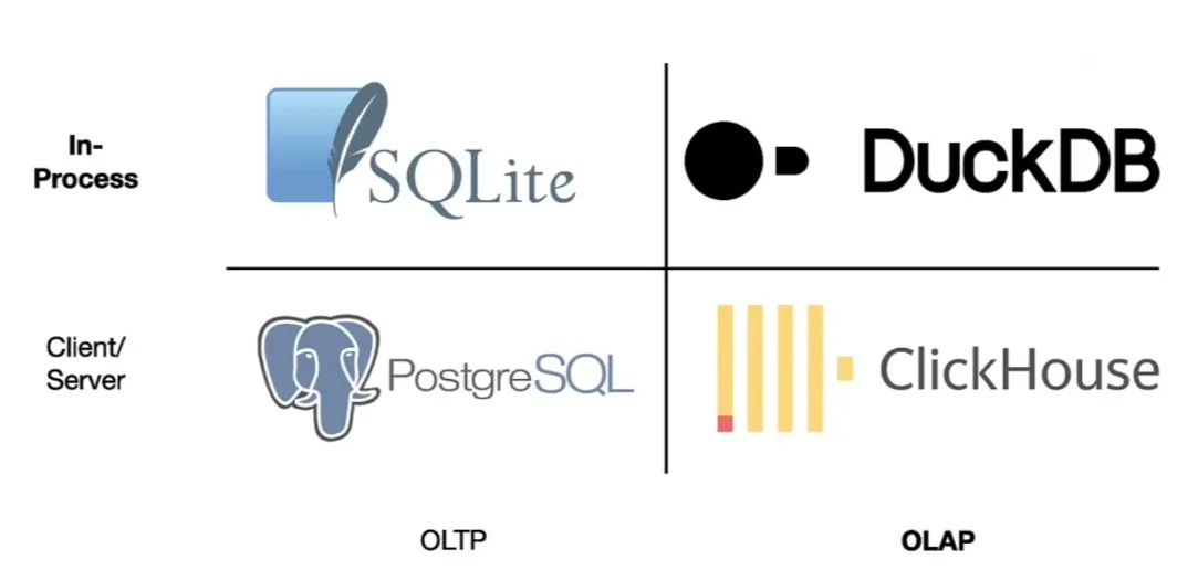
When they run into the limits of in-memory analysis in R or Python, they will instead serialize their data to local disk and use DuckDB to slam through the joins and filters that were blowing out their RAM before.
They will also take advantage of DuckDB’s ability to stream remote data from data lake object stores.
What, stream multi-gigabyte JSON files? Well, yes that’s possible, but it’s not where the action is.
The CPU is not the only laptop component that has been getting ridiculously powerful over the past few years. The network pipe that connects that laptop to the internet has also been getting both wider and lower latency with every passing year.
As the propect of streaming data for analysis has come into view, the formats for remote data have also evolved. Instead of JSON, which is relatively fluffy, and hard to efficiently filter, the Parquet format is becoming a new standard for data lakes.
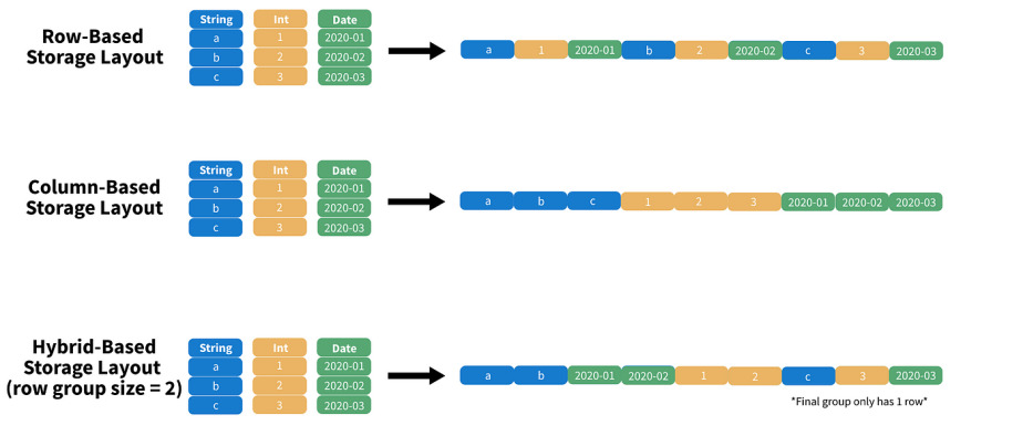
Parquet is a binary format, that organizes the data into blocks for efficient subsetting and processing. A DuckDB query to a properly organized Parquet time series file might easily pull only records for 2 of 20 columns, and 1 day of 365, reducing a multi-gigabyte download to a handful of megabytes.
The huge rise in available local computation, and network connectivity is going to spawn some new standard architectures.
Imagine a “two tier” architecture where tier one is an HTTP object store and tier two is a Javascript single page app? The COG Explorer has already been around for a few years, and it’s just such a two tier application.
(For fun, recognize that an architecture where the data are stored in an access-optimized format, and access is via primitive file-system requests, while all the smarts are in the client-side visualization software is… the old workstation GIS model. Everything old is new again.)
The technology is fresh, but the trendline is pretty clear. See Kyle Barrron’s talk about GeoParquet and DeckGL for a taste of where we are going.

Meanwhile, I expect that a lot of the growth in PostGIS / PostgreSQL we have seen in the data science field will level out for a while, as the convenience of DuckDB takes over a lot of workloads.
The limitations of Parquet (efficient remote access limited to a handful of filter variables being the primary one, as will cojoint spatial/non-spatial filter and joins) will still leave use cases that require a “real” database, but a lot of people who used to reach for PostGIS will be reaching for Duck, and that is going to change a lot of architectures, some for the better, and some for the worse.